


- If you enter a financial value complete with the dollar sign and two decimal places, Excel assigns a Currency number format to the cell along with the entry.
- If you enter a value representing a percentage as a whole number followed by the percent sign without any decimal places, Excel assigns the cell the Percentage number format that follows this pattern along with the entry.
- If you enter a date (dates are values, too) that follows one of the built-in Excel number formats, such as 11/06/13 or 06-Nov-13, the program assigns a Date number format that follows the pattern of the date along with a special value representing the date.
- Select all the cells containing the values that need dressing up.
- Select the number format that you want to use from the formatting command buttons on the Home tab or the options available on the Number tab in the Format Cells dialog box.
Even if you’re a really, really good typist and prefer to enter each value exactly as you want it to appear in the worksheet, you still have to resort to using number formats to make the values that are calculated by formulas match the others you enter. This is because Excel applies a General number format (which the Format Cells dialog box defines: “General format cells have no specific number format.”) to all the values it calculates, as well as any you enter that don’t exactly follow one of the other Excel number formats. The biggest problem with the General format is that it has the nasty habit of dropping all leading and trailing zeros from the entries. This makes it very hard to line up numbers in a column on their decimal points.
You can view this sad state of affairs in the image below, which is a sample worksheet with the first-quarter 2019 sales figures for Mother Goose Enterprises before any of the values have been formatted. Notice how the decimal in the numbers in the monthly sales figures columns zig and zag because they aren’t aligned on the decimal place. This is the fault of Excel’s General number format; the only cure is to format the values with a uniform number format.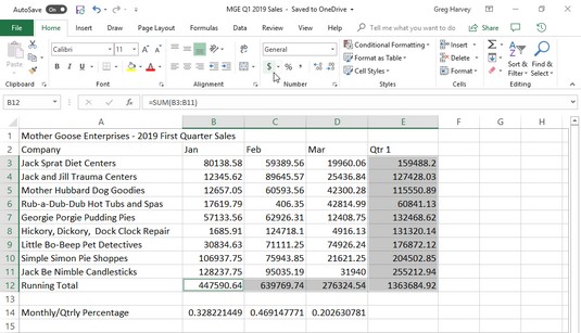 Numbers with decimals don’t align when you choose General formatting.
How to enter money in Excel 2019
Given the financial nature of most Excel 2019 worksheets, you probably use the Accounting number format more than any other. Applying this format is easy because you can assign it to the cell selection simply by clicking the Accounting Number Format button on the Home tab.The Accounting number format adds a dollar sign, commas between thousands of dollars, and two decimal places to any values in a selected range. If any of the values in the cell selection are negative, this number format displays them in parentheses (the way accountants like them). If you want a minus sign in front of your negative financial values rather than enclosing them in parentheses, select the Currency format on the Number Format drop-down menu or on the Number tab of the Format Cells dialog box.
You can see below that only the cells containing totals are selected (cell ranges E3:E10 and B10:D10). This cell selection was then formatted with the Accounting number format by simply clicking its command button (the one with the $ icon, naturally) in the Number group on the Ribbon’s Home tab.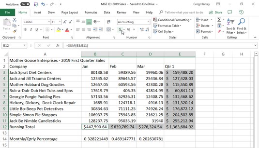 The totals in the Mother Goose sales table after clicking the Accounting Number Format button on the Home tab.
Although you could put all the figures in the table into the Accounting number format to line up the decimal points, this would result in a superabundance of dollar signs in a fairly small table. In this example, only the monthly and quarterly totals were formatted with the Accounting number format.
Excel 2019: Format overflow
When you apply the Accounting number format to the selection in the cell ranges of E3:E10 and B10:D10 in the sales table shown above, Excel adds dollar signs, commas between the thousands, a decimal point, and two decimal places to the highlighted values. At the same time, Excel automatically widens columns B, C, D, and E just enough to display all this new formatting.In versions of Excel earlier than Excel 2003, you had to widen these columns yourself, and instead of the perfectly aligned numbers, you were confronted with columns of #######s in cell ranges E3:E10 and B10:D10. Such pound signs (where nicely formatted dollar totals should be) serve as overflow indicators, declaring that whatever formatting you added to the value in that cell has added so much to the value’s display that Excel can no longer display it within the current column width.
Fortunately, Excel eliminates the format overflow indicators when you’re formatting the values in your cells by automatically widening the columns. The only time you’ll ever run across these dreaded #######s in your cells is when you take it upon yourself to narrow a worksheet column to the extent that Excel can no longer display all the characters in its cells with formatted values.
Excel 2019: Comma Style
The Comma Style format offers a good alternative to the Currency format. Like Currency, the Comma Style format inserts commas in larger numbers to separate thousands, hundred thousands, millions, and … well, you get the idea.This format also displays two decimal places and puts negative values in parentheses. What it doesn’t display is dollar signs. This makes it perfect for formatting tables where it’s obvious that you’re dealing with dollars and cents or for larger values that have nothing to do with money.
The Comma Style format also works well for the bulk of the values in the sample first-quarter sales worksheet. Check out the image below to see this table after the cells containing the monthly sales for all the Mother Goose Enterprises are formatted with the Comma Style format. To do this, select the cell range B3:D9 and click the Comma Style button — the one with the comma icon (,) — in the Number group on the Home tab.
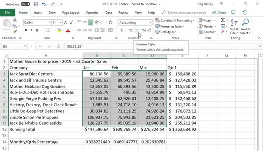 Monthly sales figures after formatting cells with the Comma Style number format.
Note how the Comma Style format in the image above takes care of the earlier decimal alignment problem in the quarterly sales figures. Moreover, Comma Style–formatted monthly sales figures align perfectly with the Currency format–styled monthly totals in row 10. If you look closely (you may need a magnifying glass for this one), you see that these formatted values no longer abut the right edges of their cells; they’ve moved slightly to the left. The gap on the right between the last digit and the cell border accommodates the right parenthesis in negative values, ensuring that they, too, align precisely on the decimal point.
Excel 2019: Percent Style
Many worksheets use percentages in the form of interest rates, growth rates, inflation rates, and so on. To insert a percentage in a cell, type the percent sign (%) after the number. To indicate an interest rate of 12 percent, for example, you enter 12% in the cell. When you do this, Excel assigns a Percentage number format and, at the same time, divides the value by 100 (that’s what makes it a percentage) and places the result in the cell (0.12 in this example).Not all percentages in a worksheet are entered by hand in this manner. Some may be calculated by a formula and returned to their cells as raw decimal values. In such cases, you should add a Percent format to convert the calculated decimal values to percentages (done by multiplying the decimal value by 100 and adding a percent sign).
The sample first-quarter-sales worksheet just happens to have some percentages calculated by formulas in row 12 that need formatting (these formulas indicate what percentage each monthly total is of the first-quarter total in cell E10). These values reflect Percent Style formatting. To accomplish this feat, you simply select the cells and click the Percent Style button in the Number group on the Home tab.
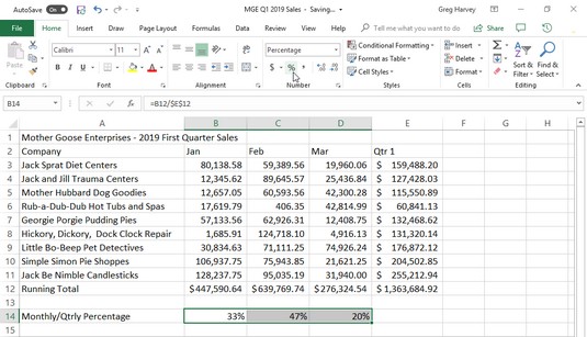 Monthly-to-quarterly sales percentages with Percentage number formatting.