How to Use the XLOOKUP Function in Excel 2016

For those of you not yet familiar with VLOOKUP (deemed the third most-used function right after SUM and AVERAGE), this function searches vertically by row in the leftmost column of a designated lookup table from top to bottom until it finds a value in a lookup column designated by an offset number that matches or exceeds the one your looking up. Although tremendously useful for locating particular items in a long list or column of a data table in your worksheet, the VLOOKUP function has several limitations not shared by this new lookup function, as XLOOKUP:

• Defaults to finding exact matches for your lookup value in the lookup range
• Can search both vertically (by row) and horizontally (by column) in a table, thereby replacing the need for using the HLOOKUP function when searching horizontally by column
• Can search left or right so that the lookup range in your lookup table does not have to be located in a column to the left of the one designated as the return range in order for the function to work
• When the exact match default is used, works even when values in the lookup range are not sorted in particular order
• Can search from the bottom row to the top in the lookup array range, using an optional search mode argument

XLOOKUP(lookup_value,lookup_array,return_array,[match_mode],[search_mode])

* Keep in mind when designating the lookup_array and return_array arguments in your XLOOKUP function, both ranges must be of equal length, otherwise Excel will return the #VALUE! error to your formula. This is all more the reason for you to use range names or column names of a designated data table when defining these arguments rather than pointing them out or typing in their cell references.

The optional match_mode argument can contain any of the following four values:

• 0 for an exact match (the default, same as when no match_mode argument is designated)
• -1 for exact match or next lesser value
• 1 for exact match or next greater value
• 2 for partial match using wildcard characters joined to cell reference in the lookup_value argument

• 1 to search first-to-last, that is, from top to bottom (the default, same as when no search_mode argument is designated)
• -1 to search last-to-first, that is, bottom to top
• 2 for a binary search in ascending order
• -2 for binary search in descending order

1. Position the cell cursor in cell E4 of the worksheet
2. Click the Lookup & Reference option on the Formulas tab followed by XLOOKUP near the bottom of the drop-down menu to open its Function Arguments dialog box.
3. Click cell D4 in the worksheet to enter its cell reference into the Lookup_value argument text box.
4. Press Tab to select the Lookup_array argument text box, then click cell A4 and hold down Shift as you press Ctrl-down arrow to select A4:A8 as the range to search (because the range A3:B8 is defined as an Excel data table, Table1[Country] appears in the text box in place of the range A4:A8).
5. Press Tab to select the Return_array argument text box, then click cell B4 and hold down Shift as you press Ctrl-down arrow to select B4:B8 as the range containing the values to be returned based on the results of the search (that appears as Table1[Total Sales] in the text box).

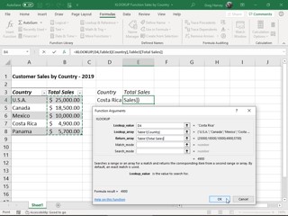Creating a formula with XLOOKUP in cell E4 that returns sales based on the country entered in cell D4.

Excel enters the XLOOKUP formula into cell E4 of the worksheet and returns 4900 as the result because Costa Rica is currently entered into the lookup cell D4 and as you can see in the 2019 sales table, this is indeed the total sales made for this country.

Because XLOOKUP works right-to-left just as well as left-to-right, you can use this function just as well to return the country from this sales table based on a particular sales figure. The following figure shows you how you do this. This time, you create the XLOOKUP formula in cell D4 and designate the value entered in cell E4 (11,000, in this case) as the lookup_value argument.

In addition, you enter -1 as the match_mode argument to override the function’s exact match default so that Excel returns the country with an exact match to the sales value entered in the lookup cell E4 or the one with the next lower total sales (Mexico with $10,000 in this case as there is no country in this table with $11,000 of total sales). Without designating a match_mode argument for this formula, Excel would return #NA as the result, because there’s no exact match to $11,000 in this sales table.

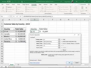Creating a formula with XLOOKUP in cell D4 that returns the country based on the sales entered in cell E4

Because the XLOOKUP function is equally comfortable searching horizontally by column as it is searching vertically by row, you can use it to create a formula the performs a two-way lookup (replacing the need to create a formula that combines the INDEX and MATCH functions as in the past). The following figure, containing the 2019 production schedule table for part numbers, AB-100 through AB-103 for the months April through December, shows you how this is done.

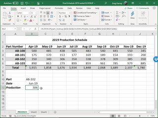Creating a formula with nested XLOOKUP functions to return the number of units produced for a part in a particular month

In cell B12, I created the following formula:

=XLOOKUP(part_lookup,$A$3:$A$6,XLOOKUP(date_lookup,$B$2:$J$2,$B$3:$J$6))

This second, nested XLOOKUP function searches the cell range $B$2:$J$2 horizontally by column for an exact match to the date entry made in the cell named date_lookup (cell B11, in this case). The return_array argument for this second, nested XLOOKUP function is $B$3:$J$6, the cell range of all production values in the table.

The way this formula works is that Excel first calculates the result of the second, nested XLOOKUP function by performing a horizontal search that, in this case, returns the array in cell range D3: D6 of the Jun-19 column (with the values: 438, 153, 306, and 779) as its result. This result, in turn, becomes the return_array argument for the original XLOOKUP function that performs a vertical search by row for an exact match to the part number entry made in cell B11 (named part_lookup). Because, in this example, this part_lookup cell contains AB-102, the formula returns just the Jun-19 production value, 306, from the result of the second, next XLOOKUP function.

There you have it! A first look at XLOOKUP, a powerful, versatile, and fairly easy-to-use new lookup function that can not only do the single-value lookups performed by the VLOOKUP and HLOOKUP functions but also the two-way value lookups performed by combining the INDEX and MATCH functions as well.

* Unfortunately, the XLOOKUP function is not backward compatible with earlier versions of Microsoft Excel that only support the VLOOKUP and HLOOKUP functions or compatible with current versions that do not yet include it as one of their lookup functions, such as Excel 2019 and Excel Online. This means that if you share a workbook containing XLOOKUP formulas with co-workers or clients who are using a version of Excel that doesn’t include this new lookup function, all these formulas will return #NAME? error values when they open its worksheet.