


Rattle provides a GUI to R’s tree-construction and tree-plotting functions. To use this GUI to create a decision tree for iris.uci, begin by opening Rattle:library(rattle)
rattle()
The information here assumes that you’ve downloaded and cleaned up the iris dataset from the UCI ML Repository and called it iris.uci.
On Rattle’s Data tab, in the Source row, click the radio button next to R Dataset. Click the down arrow next to the Data Name box and select iris.uci from the drop-down menu. Then click the Execute icon in the upper left corner.
If you haven’t downloaded the UCI iris dataset and you just want to use the iris dataset that comes with base R, click the Library radio button. Then click the down arrow next to the Data Name box and select
iris:datasets:Edgar Anderson’s iris datafrom the drop-down menu. Then click Execute.
You probably want to try downloading from UCI, though, to get the hang of it. Downloading from the UCI ML Repository is something you’ll be doing a lot.
Still on the Data tab, select the Partition check box. This breaks down the dataset into a training set, a validation set, and a test set. The default proportions are 70 percent training, 15 percent validation, and 15 percent test. The idea is to use the training set to construct the tree and then use the test set to test its classification rules. The validation set provides a set of cases to experiment with different variables or parameters. Because you don’t do that in this example, you set the percentages to 70 percent training, 0 percent validation, and 30 percent test.
The Seed box contains a default value, 42, as a seed for randomly assigning the dataset rows to training, validation, or testing. Changing the seed changes the randomization.
Creating the tree
Decision tree modeling resides on the Model tab. It opens with Tree selected.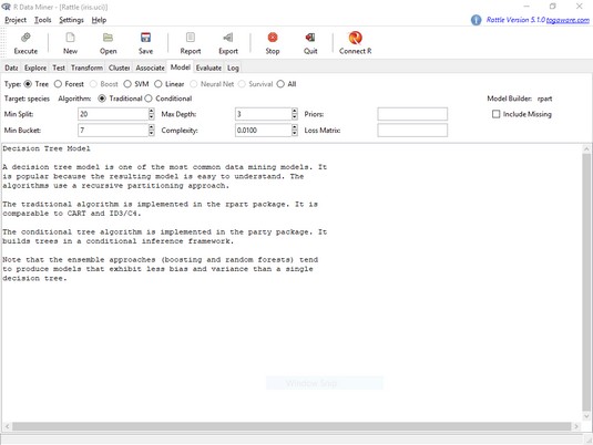 The
The Rattle Model tab.A number of onscreen boxes provide access to rpart()’s arguments. (These are called tuning parameters.) Moving the cursor over a box opens helpful messages about what goes in the box.
For now, just click Execute to create the decision tree.
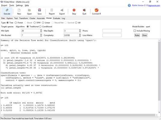
The text in the main panel is output from rpart(). Note that the tree is based on the 105 cases (70 percent of 150) that constitute the training set. Unlike the tree created earlier, this one just uses petal.length in its splits.
The rest of the output is from a function called printcp(). The abbreviation cp stands for complexity parameter, which controls the number of splits that make up the tree. Without delving too deeply into it, you just need to know that if a split adds less than the given value of cp (on the Model tab, the default value is .01), rpart() doesn’t add the split to the tree. For the most complex tree possible (with the largest number of possible splits, in other words), set cp to .00.
 The
The Rattle Model tab, after creating a decision tree for iris.uci.Drawing the tree
Clicking the Draw button produces the decision tree shown below, rendered byprp(). The overall format of the tree is similar to the tree shown earlier, although the details are different and the boxes at the nodes have fill color.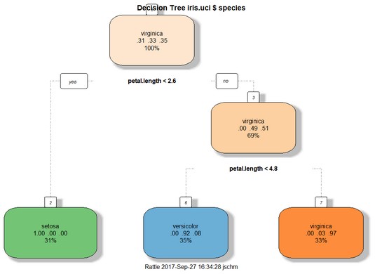 A decision tree for
 iris.uci, based on a training set of 105 cases.Evaluating the tree
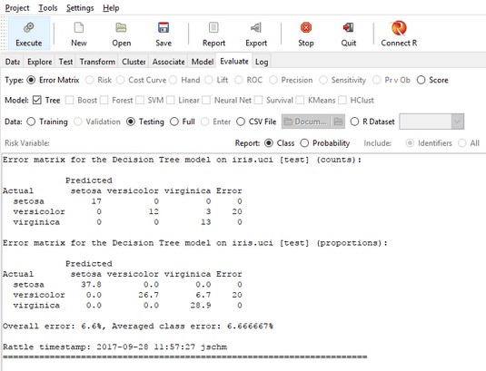
The idea behind evaluation is to assess the performance of the tree (derived from the training data) on a new set of data. This is why the data is divided into a Training set and a Testing set.To see how well the decision tree performs, select the Evaluate tab. The image below shows the appearance of the tab after clicking Execute with the default settings (which are appropriate for this example).
The results of the evaluation for the 45 cases in the Testing set (30 percent of 150) appear in two versions of an error matrix. Each row of a matrix represents the actual species of the flower. Each column shows the decision tree’s predicted species of the flower. The first version of the matrix shows the results by counts; the second, by proportions.
Correct identifications are in the main diagonal. So in the first matrix, the cell in row 1, column 1 represents the number of times the decision tree correctly classified a setosa as a setosa (17). The zeros in the other two cells in row 1 indicate no misclassified setosas.
 The
The Rattle Evaluate tab, after evaluating the decision tree for iris.uci.The cell in row 2, column 3 shows that the tree incorrectly classified three virginicas as versicolors. The fourth column shows that the error rate is 20 percent (3/(12 + 3)).
Row 3 shows no misclassifications, so dividing the 20 percent by 3 (the number of categories) gives the averaged class error you see at the bottom. The overall error is the number of misclassifications divided by the total number of observations.
