


Using natural logs for variables on both sides of your econometric specification is called a log-log model. This model is handy when the relationship is nonlinear in parameters, because the log transformation generates the desired linearity in parameters (you may recall that linearity in parameters is one of the OLS assumptions).
In principle, any log transformation (natural or not) can be used to transform a model that’s nonlinear in parameters into a linear one. All log transformations generate similar results, but the convention in applied econometric work is to use the natural log. The practical advantage of the natural log is that the interpretation of the regression coefficients is straightforward.
Consider the demand function
where Q is the quantity demanded, alpha is a shifting parameter, P is the price of the good, and the parameter beta is less than zero for a downward-sloping demand curve.
you can recognize the function as a specific type of demand curve with elasticity equal to –1 at all points; that is, you have a unitary elastic demand curve.
A demand curve of the form
has a constant elasticity, but the value of that elasticity may not be known. Using data, you can estimate the parameters, but you must transform the function in order to make estimates using the OLS technique.
If your model is not linear in parameters, sometimes a log transformation achieves linearity.
A generic form of a constant elasticity model can be represented by
If you take the natural log of both sides, you end up with
You treat
as the intercept. You end up with the following model:
You can estimate this model with OLS by simply using natural log values for the variables instead of their original scale.
After estimating a log-log model, such as the one in this example, the coefficients can be used to determine the impact of your independent variables (X) on your dependent variable (Y). The coefficients in a log-log model represent the elasticity of your Y variable with respect to your X variable. In other words, the coefficient is the estimated percent change in your dependent variable for a percent change in your independent variable.
Using calculus with a simple log-log model, you can show how the coefficients should be interpreted. Begin with the model
and differentiate it to obtain
The term on the right-hand side is the percent change in X, and the term on the left-hand side is the percent change in Y, so
measures the elasticity.
Suppose you obtain the estimates
where Y is sales and X is price. The elasticity is –0.85, so a 1 percent increase in the price is associated with a 0.85 percent decrease in quantity demanded (sales), on average.
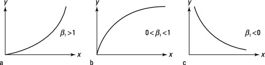
If you estimate a log-log regression, a few outcomes for the coefficient on X produce the most likely relationships:
Part (a) shows this log-log function in which the impact of the independent variable is positive and becomes larger as its value increases.
Part (b) shows a log-log function in which the impact of the independent variable is positive but becomes smaller as its value increases.
Part (c) shows a log-log function where the impact of the dependent variable is negative.
Although regression coefficients are sometimes referred to as partial-slope coefficients, in a log-log model the coefficients don’t represent the slope (or unit change in your Y variable for a unit change in your X variable).
