


If the column headings of your data list table don’t currently have filter drop-down buttons displayed in their cells after the field names, you can add them simply by clicking Home → Sort & Filter → Filter or pressing Alt+HSF. (Check out these other entry and formatting shortcuts.)
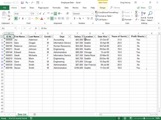
For example, in the image below, the Employee Data List was filtered to display only those records in which the Location is either Boston or San Francisco by clicking the Location field’s AutoFilter button and then clicking the (Select All) check box to remove its check mark. Then, the Boston and San Francisco check boxes were selected to add check marks to them before clicking OK. (It’s as simple as that.)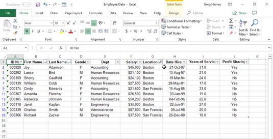 The Employee Data List after Excel filters out all records except those with Boston or San Francisco in the Location field.
After you filter a data list so that only the records you want to work with are displayed, you can copy those records to another part of the worksheet to the right of the database (or better yet, another Excel sheet in the workbook). Simply select the cells, then click the Copy button on the Home tab or press Ctrl+C, move the cell cursor to the first cell where the copied records are to appear, and then press Enter. After copying the filtered records, you can then redisplay all the records in the database or apply a slightly different filter.
If you find that filtering the data list by selecting a single value in a field drop-down list box gives you more records than you really want to contend with, you can further filter the database by selecting another value in a second field’s drop-down list.For example, suppose that you select Boston as the filter value in the Location field’s drop-down list and end up with hundreds of Boston records displayed in the worksheet. To reduce the number of Boston records to a more manageable number, you could then select a value (such as Human Resources) in the Dept field’s drop-down list to further filter the database and reduce the records you have to work with onscreen. When you finish working with the Boston Human Resources employee records, you can display another set by displaying the Dept field’s drop-down list again and changing the filter value from Human Resources to some other department, such as Accounting.
When you’re ready to display all the records in the database again, click the filtered field’s AutoFilter button (indicated by the appearance of a cone filter on its drop-down button) and then click the Clear Filter from (followed by the name of the field in parentheses) option near the middle of its drop-down list.
You can temporarily remove the AutoFilter buttons from the cells in the top row of the data list containing the field names and later redisplay them by clicking the Filter button on the Data tab or by pressing Alt+AT or Ctrl+Shift+L. You can also use Slicer and Timeline filters on your data.
Using Excel’s ready-made number filters: Top 10
Excel contains a number filter option called Top 10. You can use this option on a number field to show only a certain number of records (like the ones with the ten highest or lowest values in that field or those in the ten highest or lowest percent in that field or just those that are above or below average of that field).To use the Top 10 option in Excel to filter a database, follow these steps:
- Click the AutoFilter button on the numeric field you want to filter with the Top 10 option. Then highlight Number Filters in the drop-down list and click Top 10 on its submenu.Excel opens the Top 10 AutoFilter dialog box. By default, the Top 10 AutoFilter chooses to show the top ten items in the selected field. However, you can change these default settings before filtering the database.
- To show only the bottom ten records, change Top to Bottom in the left-most drop-down list box.
- To show more or fewer than the top or bottom ten records, enter the new value in the middle text box (that currently holds 10) or select a new value by using the spinner buttons.
- To show those records that fall into the Top 10 or Bottom 10 (or whatever) percent, change Items to Percent in the right-most drop-down list box.
- Click OK or press Enter to filter the database by using your Top 10 settings.
In the image below, you can see the Employee Data List after using the Top 10 option (with all its default settings) to show only those records with salaries that are in the top ten. David Letterman would be proud!
 The Employee Data List after using the Top 10 AutoFilter to filter out all records except for those with the ten highest salaries.
Using Excel’s ready-made date filters
When filtering a data list by the entries in a date field, Excel makes available a variety of date filters that you can apply to the list. These ready-made filters include Equals, Before, After, and Between as well as Tomorrow, Today, Yesterday, as well as Next, This, and Last for the Week, Month, Quarter, and Year. Additionally, Excel offers Year to Date and All Dates in the Period filters. When you select the All Dates in the Period filter, Excel enables you to choose between Quarter 1 through 4 or any of the 12 months, January through December, as the period to use in filtering the records.To select any of these date filters, you click the date field’s AutoFilter button, then highlight Date Filters on the drop-down list and click the appropriate date filter option on the continuation menu(s).
Using custom autofilters in Excel 2019
In addition to filtering a data list to records that contain a particular field entry (such as Newark as the City or CA as the State), you can create custom AutoFilters that enable you to filter the list to records that meet less-exacting criteria (such as last names starting with the letter M) or ranges of values (such as salaries between $25,000 and $75,000 a year).To create a custom filter for a field, you click the field’s AutoFilter button and then highlight Text Filters, Number Filters, or Date Filters (depending on the type of field) on the drop-down list and then click the Custom Filter option at the bottom of the continuation list. When you select the Custom Filter option, Excel displays a Custom AutoFilter dialog box.
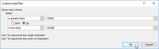 Use a custom AutoFilter to display records with entries in the Salary field between $25,000 and $75,000.
You can also open the Custom AutoFilter dialog box by clicking the initial operator (Equals, Does Not Equal, Greater Than, and so on) on the field’s Text Filters, Number Filters, or Date Filters submenus.
In this dialog box, you select the operator that you want to use in the first drop-down list box. Then enter the value (text or numbers) that should be met, exceeded, fallen below, or not found in the records of the database in the text box to the right.| Operator | Example | What It Locates in the Database |
| Equals | Salary equals 35000 | Records where the value in the Salary field is equal to $35,000 |
| Does not equal | State does not equal NY | Records where the entry in the State field is not NY (New York) |
| Is greater than | Zip is greater than 42500 | Records where the number in the Zip field comes after 42500 |
| Is greater than or equal to | Zip is greater than or equal to 42500 | Records where the number in the Zip field is equal to 42500 or comes after it |
| Is less than | Salary is less than 25000 | Records where the value in the Salary field is less than $25,000 a year |
| Is less than or equal to | Salary is less than or equal to 25000 | Records where the value in the Salary field is equal to $25,000 or less than $25,000 |
| Begins with | Begins with d | Records with specified fields have entries that start with the letter d |
| Does not begin with | Does not begin with d | Records with specified fields have entries that do not start with the letter d |
| Ends with | Ends with ey | Records whose specified fields have entries that end with the letters ey |
| Does not end with | Does not end with ey | Records with specified fields have entries that do not end with the letters ey |
| Contains | Contains Harvey | Records with specified fields have entries that contain the name Harvey |
| Does not contain | Does not contain Harvey | Records with specified fields have entries that don’t contain the name Harvey |
To set up a range of values, you select the “is greater than” or “is greater than or equal to” operator for the top operator and then enter or select the lowest (or first) value in the range. Then, make sure that the And option is selected, select “is less than” or “is less than or equal to” as the bottom operator, and enter the highest (or last) value in the range.
Check out the images above and below to see how Excel filters the records in the Employee Data List so that only those records where Salary amounts are between $25,000 and $75,000 are displayed. As shown above, you set up this range of values as the filter by selecting “is greater than or equal to” as the operator and 25,000 as the lower value of the range. Then, with the And option selected, you select “is less than or equal to” as the operator and 75,000 as the upper value of the range. The results of applying this filter to the Employee Data List are shown below.
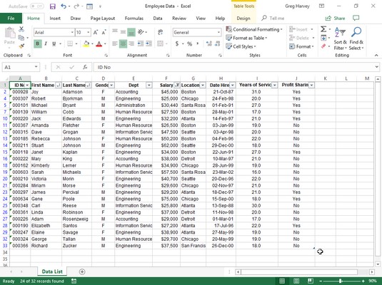 The Employee Data List after applying the custom AutoFilter.
To set up an either/or condition in the Custom AutoFilter dialog box, you normally choose between the “equals” and “does not equal” operators (whichever is appropriate) and then enter or select the first value that must be met or must not be equaled. Then you select the Or option and select whichever operator is appropriate and enter or select the second value that must be met or must not be equaled.
For example, if you want Excel to filter the data list so that only records for the Accounting or Human Resources departments in the Employee Data List appear, you select “equals” as the first operator and then select or enter Accounting as the first entry. Next, you click the Or option, select “equals” as the second operator, and then select or enter Human Resources as the second entry. When you then filter the database by clicking OK or pressing Enter, Excel displays only those records with either Accounting or Human Resources as the entry in the Dept field.


