


If you just need to copy a single formula in Excel 2016, use the AutoFill feature or the Copy and Paste commands. This type of formula copy, although quite common, can't be done with drag and drop.
Don't forget the Totals option on the Quick Analysis tool. You can use it to create a row or a column of totals at the bottom or right edge of a data table in a flash. Simply select the table as a cell range and click the Quick Analysis button followed by Totals in its palette. Then click the Sum button at the beginning of the palette to create formulas that total the columns in a new row at the bottom of the table and/or the Sum button at the end of the palette to create formulas that total the rows in a new column at the right end.
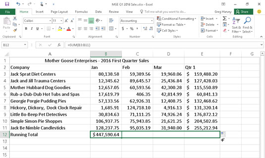
Here's how you can use AutoFill to copy one formula to a range of cells. In this figure, you can see the Mother Goose Enterprises – 2016 Sales worksheet with all the companies, but this time with only one monthly total in row 12, which is in the process of being copied through cell E12.
The following figure shows the worksheet after dragging the fill handle in cell B12 to select the cell range C12:E12 (where this formula should be copied).
Relatively speaking
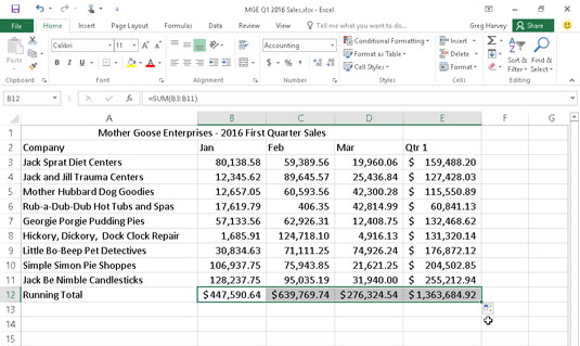
The figure shows the worksheet after the formula in a cell is copied to the cell range C12:E12 and cell B12 is active. Notice how Excel handles the copying of formulas. The original formula in cell B12 is as follows:
=SUM(B3:B11)
When the original formula is copied to cell C12, Excel changes the formula slightly so that it looks like this:
=SUM(C3:C11)
Excel adjusts the column reference, changing it from B to C, because you copied from left to right across the rows.
When you copy a formula to a cell range that extends down the rows, Excel adjusts the row numbers in the copied formulas rather than the column letters to suit the position of each copy. For example, cell E3 in the Mother Goose Enterprises – 2016 Sales worksheet contains the following formula:
=SUM(B3:D3)
When you copy this formula to cell E4, Excel changes the copy of the formula to the following:
=SUM(B4:D4)
Excel adjusts the row reference to keep current with the new row 4 position. Because Excel adjusts the cell references in copies of a formula relative to the direction of the copying, the cell references are known as relative cell references.
Some things are absolutes!
All new formulas you create naturally contain relative cell references unless you say otherwise. Because most copies you make of formulas require adjustments of their cell references, you rarely have to give this arrangement a second thought. Then, every once in a while, you come across an exception that calls for limiting when and how cell references are adjusted in copies.
One of the most common of these exceptions is when you want to compare a range of different values with a single value. This happens most often when you want to compute what percentage each part is to the total. For example, in the Mother Goose Enterprises – 2016 Sales worksheet, you encounter this situation in creating and copying a formula that calculates what percentage each monthly total (in the cell range B14:D14) is of the quarterly total in cell E12.
Suppose that you want to enter these formulas in row 14 of the Mother Goose Enterprises – 2016 Sales worksheet, starting in cell B14. The formula in cell B14 for calculating the percentage of the January-sales-to-first-quarter-total is very straightforward:
=B12/E12
This formula divides the January sales total in cell B12 by the quarterly total in E12 (what could be easier?). Look, however, at what would happen if you dragged the fill handle one cell to the right to copy this formula to cell C14:
=C12/F12
The adjustment of the first cell reference from B12 to C12 is just what the doctor ordered. However, the adjustment of the second cell reference from E12 to F12 is a disaster. Not only do you not calculate what percentage the February sales in cell C12 are of the first quarter sales in E12, but you also end up with one of those horrible #DIV/0! error things in cell C14.
To stop Excel from adjusting a cell reference in a formula in any copies you make, convert the cell reference from relative to absolute. You do this by pressing the function key F4, after you put Excel in Edit mode (F2). Excel indicates that you make the cell reference absolute by placing dollar signs in front of the column letter and row number. For example, in this figure, cell B14 contains the correct formula to copy to the cell range C14:D14:
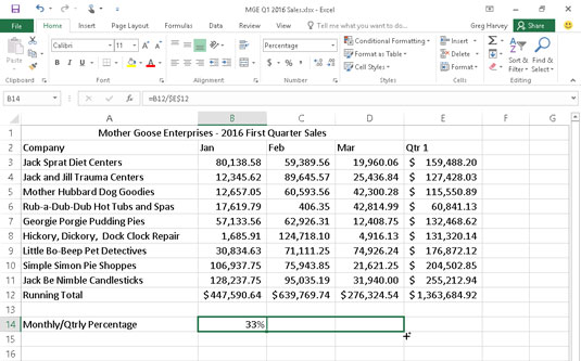
=B12/$E$12
Look at the worksheet after this formula is copied to the range C14:D14 with the fill handle and cell C14 is selected (see the following figure). Notice that the Formula bar shows that this cell contains the following formula:
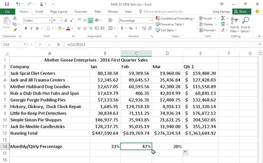
=C12/$E$12
Because E12 was changed to $E$12 in the original formula, all the copies have this same absolute (non-changing) reference.
If you goof up and copy a formula where one or more of the cell references should have been absolute but you left them all relative, edit the original formula as follows:
Double-click the cell with the formula or press F2 to edit it.
Position the insertion point somewhere on the reference you want to convert to absolute.
Press F4.
When you finish editing, click the Enter button on the Formula bar and then copy the formula to the messed-up cell range with the fill handle.
Be sure to press F4 only once to change a cell reference to completely absolute as I describe earlier. If you press the F4 function key a second time, you end up with a so-called mixed reference, where only the row part is absolute and the column part is relative (as in E$12). If you then press F4 again, Excel comes up with another type of mixed reference, where the column part is absolute and the row part is relative (as in $E12). If you go on and press F4 yet again, Excel changes the cell reference back to completely relative (as in E12).
After you're back where you started, you can continue to use F4 to cycle through this same set of cell reference changes all over again.
If you're using Excel 2016 on a device without access to a physical keyboard with function keys (such as a touchscreen tablet), the only way to convert cell addresses in your formulas from relative to absolute or some form of mixed address is to open the Touch keyboard and use it add the dollar signs before the column letter and/or row number in the appropriate cell address on the Formula bar.


