


When enacting a Six Sigma initiative, you will undoubtedly encounter short term variation. Short-term variation is purely random. Like rolling a pair of dice, you can’t predict what the next output value will be. If you could, Las Vegas would be bankrupt in a week!
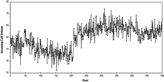
Suppose you monitor a characteristic of a product or process — say, the volume of inbound calls per hour at a customer call center — over an extended period. After each hour, you measure and record the number of calls received. To review what you’ve observed, you graph your collected measurements as a sequence of connected points along an axis representing time.
Although the points graphed represent the number of incoming calls per hour, recognize that they can also represent any process characteristic in any type of company. All process characteristics vary from cycle to cycle: the exact length of newly manufactured pencils, the time required to fill out an invoice, the number of calls per hour, and so on.
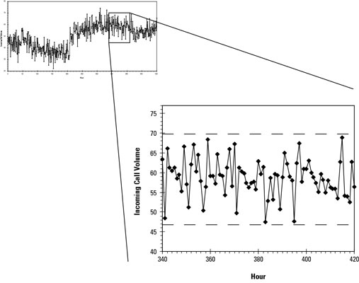
If you zoom in on a narrow portion of the graph, you can see from the scattered points that the output certainly does vary for each measurement cycle. But you can also notice that the variation isn’t limitless. It lies within upper and lower boundary limits — represented by the dashed, horizontal lines.
In fact, for any selected short period of time, the process essentially varies within the same rough limits. This natural level of variation is called the short-term variation of a process. Often, it’s designated with a simple ST notation.
Short-term variation is what you use to compare the inherent capability of different processes to meet a specified goal.
For example, creating a shaped plastic part by using an injection mold machine may have an entitlement variation of ±0.002 inches. The process of cutting plastic with a milling machine, on the other hand, may have an entitlement variation of ±0.0005 inches. In this case, the milling machine process has the better level of entitlement. It has less inherent, short-term variation.
The many mini-causes of short-term variation
Short-term variation is caused by the combined effect of all the little things that are too hard to include in your understanding of the process. It is too difficult to determine exactly how the microscopic textures of the dice contribute to their spin as they contact the felt surface of the table, or how the drag of the swirling air on the corners of the airborne dice alters their tumble.
The reality of short-term variation in any and all processes, from rolling dice to preparing a meal to writing a memo to launching a rocket, is that the complete chain of causation is unknown and unknowable. Like rolling dice, your ability to understand the full depth of causation for any process is ultimately limited.
Because these small forces are present to some degree in all processes, they’re referred to as common. Consequently, the short-term variation they cause is sometimes called common cause variation.
How to calculate short-term variation
After you know what short-term variation is, you need to know how to quantify it. The formula for calculating the standard deviation doesn’t account for any short- or long-term effects. It just looks at the overall variation in all the measurements. But never fear; hard-working statisticians have developed a way to extract the level of the short-term variation out from the overall variation.
The quickest way to get to the short-term variation is to analyze the separation or differences between sequential measurements of a critical characteristic. The difference between any two sequential measurements can be thought of as a kind of range. For a sequence of measurements
x1, x2, . . . xn–1, xn
where n is the total number of collected data points, you can write the difference or range between the first and second measurements as
In general, the difference between any two sequential measurements is
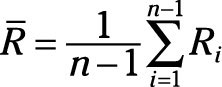
The vertical parentheses-like bars in the equation are called an absolute value. They signal you to take the positive magnitude of the calculated difference inside the absolute value symbols, regardless of whether it is a positive or negative value. And the average range or difference between sequential points is
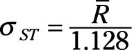
The way to calculate the short-term standard deviation from these sequential, between-point ranges is to multiply their average by a special correction factor based on the range between two sequential measurements:
Never try to calculate a characteristic’s short-term standard deviation on anything but a sequential set of measurements. Only perform this calculation on a set of measurements that are in the exact order that the measurements were taken. The calculation of the short-term standard deviation is based on the natural ranges that occur between the characteristic’s measurements; altering the order of the measurements in any way affects the short-term standard deviation.


