The value field settings for a pivot table determine what Excel does with a field when it’s cross-tabulated in the pivot table. This process sounds complicated, but this quick example shows you exactly how it works. If you right-click one of the sales revenue amounts shown in the pivot table and choose Value Field Settings from the shortcut menu that appears, Excel displays the Value Field Settings dialog box.
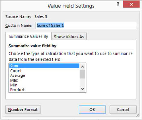
Using the Summarize Values By tab of the Data Field Settings dialog box, you can indicate whether the data item should be summed, counted, averaged, and so on, in the pivot table. By default, data items are summed. But you can also arithmetically manipulate data items in other ways. For example, you can calculate average sales by selecting Average from the list box.
You can also find the largest value by using the Max function, the smallest value by using the Min function, the number of sales transactions by using the Count function, and so on. Essentially, what you do with the Data Field Settings dialog box is pick the arithmetic operation that you want Excel to perform on data items stored in the pivot table.
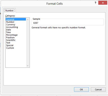
If you click the Number Format button in the Data Field Settings dialog box, Excel displays a scaled-down version of the Format Cells dialog box. From the Format Cells dialog box, you can pick a numeric format for the data item.
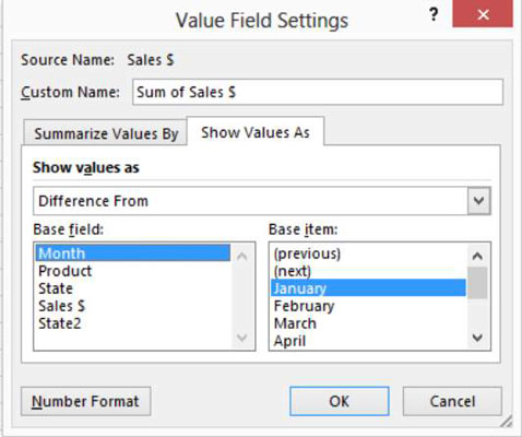
Click the Show Values As tab of the Value Field Settings dialog box, and Excel provides several additional boxes that enable you to specify how the data item should be manipulated for fancy-schmancy summaries.