


The Chart Title and Axis Titles commands, which appear when you click the Design tab’s Add Chart Elements command button in Excel, let you add a title to your chart titles to the vertical, horizontal, and depth axes of your chart.
In Excel 2007 and Excel 2010, you use the Chart Title and Axis Titles commands on the Layout tab to add chart and axis titles.
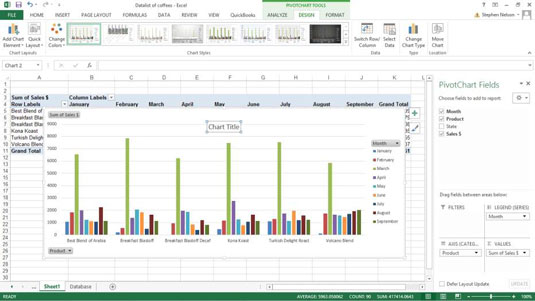
After you choose the Chart Title or Axis Title command, Excel displays a submenu of commands you use to select the title location. After you choose one of these location-related commands, Excel adds a placeholder box to the chart. This chart shows the placeholder added for a chart title. To replace the placeholder title text, click the placeholder and type the title you want.
If you click the chart title once you’ve replaced the placeholder, Excel opens a Format Chart Title pane along the right edge of the Excel program window. This pane provides buttons you can use to control the appearance of the title and the box the title sits in.
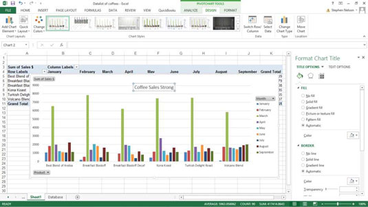
The Format Chart Title pane, for example, provides a set of Fill options that let you fill in the chart title box with color or a pattern. (If you do select a fill color or pattern, Excel adds buttons and boxes to the set of Fill options so you can specify what the color or pattern should be.)
The Format Chart Title pane provides buttons and boxes for you to specify how you want any lines drawn or fill for the title or its box to look in terms of thickness, color, and style. The pane provides buttons and boxes for specifying any special effects, including shadowing, glow, edge softening, and the illusion of three-dimensionality. You can also control the sizing and setting other properties of the title.
You click the little icons at the top of a pane to flip between the different settings a pane supplies. In the case of the Format Chart Title pane, for example, you click the icons that look like a paint can, a pentagon and a box with measurement marks to access the Fill & Line, the Effects and then the Size & Properties settings.
Different Excel formatting panes provide different sets of formatting options. So go ahead and experiment with your options here to get comfortable with the options you have for your pivot charts.
In Excel 2007 and Excel 2010, you use the Format Chart Title dialog box rather than the Format Chart Title pane to customize the appearance of the chart title. To display the Format Chart Title dialog box, click the Layout tab’s Chart Title command button and then choose the More Title Options command from the menu Excel displays.
