


In case you haven’t noticed, graphic objects in Excel 2013 float on top of the cells of the worksheet and may need some controlling. Most of the objects are opaque, meaning that they hide information in the cells beneath.
If you move one opaque graphic so that it overlaps part of another, the one on top hides the one below, just as putting one sheet of paper partially on top of another hides some of the information on the one below. Most of the time, you should make sure that graphic objects don’t overlap one another or overlap cells with worksheet information that you want to display.
How to reorder the layering of graphic objects
When graphic objects (including charts, text boxes, inserted clip art and pictures, drawn shapes, and SmartArt graphics) overlap each other, you can change how they overlay each other by sending the objects back or forward so that they reside on different (invisible) layers.
Excel 2013 enables you to move a selected graphic object to a new layer in one of two ways:
To move the selected object up toward or to the top layer, select the Bring Forward or Bring to Front option on the Bring Forward button’s drop-down menu in the Arrange group on object’s Drawing, Pictures, or SmartArt Tools contextual tab.
To move the selected object down toward or to the bottom layer, select the Send Backward or Send to Back option on the Send Backward button’s drop-down menu in the Arrange group on object’s Drawing, Pictures, or SmartArt Tools contextual tab.
Click the Selection Pane command button in the Arrange group on the Format tab under the Drawing Tools, Pictures Tools, or SmartArt Tools contextual tab to display the Selection task pane. Click the Bring Forward button or Send Backward button at the top to the immediate right of the Show All and Hide All buttons. Click until the selected graphic object appears on the desired layer.
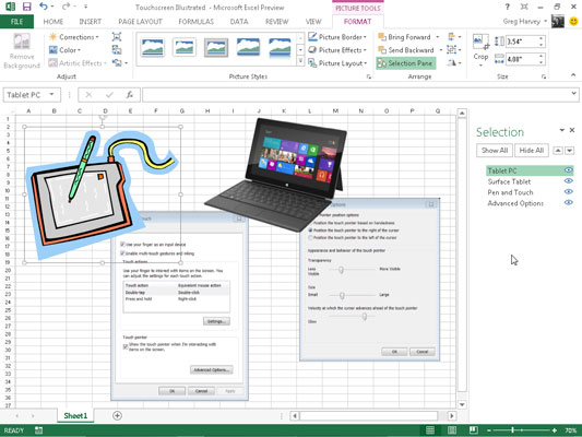
Here you have a combination of downloaded clip art, web picture, and screenshot graphic, along with a drawn graphic object on the same worksheet but on different layers. As you can see in the Selection task pane, the Tablet PC clip art image is on the topmost layer so that it would obscure any of the other three graphic objects on layers below that it happens to overlap.
Next comes the picture of the Microsoft Surface Tablet on the second graphics layer so it obscures part of the drawn Explosion Graphic and the Mouse Properties dialog box screenshot graphic that ware placed on the third and fourth graphics layers, respectively. To move these graphic objects to a new layer, you have only to select them in the Selection pane followed by the Bring Forward or Send Backward buttons.
How to group graphic objects
Sometimes you may find that you need to group several graphic objects so that they act as one unit. That way, you can move these objects or size them in one operation.
To group objects, Ctrl+click each object you want to group to select them all. Next, click the Group Objects button in the Arrange group on the Format tab under the appropriate Tools and then click Group on its drop-down menu.
After grouping several graphic objects, whenever you click any part of the mega-object, every part is selected (and selection handles appear only around the perimeter of the combined object).
If you need to independently move or size grouped objects, you can ungroup them by right-clicking an object and then choosing Group→Ungroup on the object’s shortcut menu or by clicking Group→Ungroup on the Format tab under the appropriate Tools contextual tabs.
How to hide graphic objects
The Selection task pane enables you to change the layering of various graphic objects in the worksheet, and to control whether they are hidden or displayed. To open the Selection task pane, select one of the graphic objects on the worksheet and then click the Format button under the respective Tools contextual tab. Click the Selection Pane button found in the Arrange group of the object’s Format tab.
After you open the Selection task pane, you can temporarily hide any of the graphic objects listed by clicking its eye check box. To remove the display of all the charts and graphics in the worksheet, click the Hide All button at the top task pane instead.
To redisplay a hidden graphic object, simply click its empty eye check box to put the eye icon back into it. To redisplay all graphic objects after hiding them all, click the Show All button at the top of the task pane.
If you hide all the charts and graphics in a worksheet by clicking the Hide All button and then close the Selection task pane by clicking its Close button, you’ll have no way of redisplaying this task pane so that you can bring back their display by clicking the Show All button.
That’s because you have no visible graphic objects left to select in the worksheet and, therefore, no way to get the contextual tabs with their Selection Pane buttons to appear on the Ribbon.
In this dire case, the only way to get the Selection task pane to appear so that you can click the Show All button is to create a dummy graphic object in the worksheet. Then click the Selection Pane button on the Format tab of its Drawing Tools contextual tab.
With the Selection task pane open, click the Show All button to bring back the display of all the charts and graphics you want to keep. Get rid of the still-selected dummy graphic object by pressing the Delete key.
