10 Ways to Improve Power Pivot Performance

One huge influence on Power Pivot performance is the number of columns you bring, or import, into the data model. Every column you import is one more dimension that Power Pivot has to process when loading a workbook. Don’t import extra columns “just in case” — if you’re not certain you will use certain columns, just don’t bring them in. These columns are easy enough to add later if you find that you need them.

More rows mean more data to load, more data to filter, and more data to calculate. Avoid selecting an entire table if you don’t have to. Use a query or a view at the source database to filter for only the rows you need to import. After all, why import 400,000 rows of data when you can use a simple WHERE clause and import only 100,000?

Speaking of views, for best practice, use views whenever possible.

Though tables are more transparent than views — allowing you to see all the raw, unfiltered data — they come supplied with all available columns and rows, whether you need them or not. To keep your Power Pivot data model to a manageable size, you’re often forced to take the extra step of explicitly filtering out the columns you don’t need.

Views can not only provide cleaner, more user-friendly data but also help streamline your Power Pivot data model by limiting the amount of data you import.

Both the number of relationships and the number of relationship layers have an impact on the performance of your Power Pivot reports. When building your model, follow best practice and have a single fact table containing primarily quantitative numerical data (facts) and dimension tables that relate to the facts directly. In the database world, this configuration is a star schema, as shown.

Avoid building models where dimension tables relate to other dimension tables.

Most Excel analysts who are new to Power Pivot tend to pull raw data directly from the tables on their external database servers. After the raw data is in Power Pivot, they build calculated columns and measures to transform and aggregate the data as needed. For example, users commonly pull revenue and cost data and then create a calculated column in Power Pivot to compute profit.

So why make Power Pivot do this calculation when the back-end server could have handled it? The reality is that back-end database systems such as SQL Server have the ability to shape, aggregate, clean, and transform data much more efficiently than Power Pivot. Why not utilize their powerful capabilities to massage and shape data before importing it into Power Pivot?

Rather than pull raw table data, consider leveraging queries, views, and stored procedures to perform as much of the data aggregation and crunching work as possible. This leveraging reduces the amount of processing that Power Pivot will have to do and naturally improves performance.

Columns that have a high number of unique values are particularly hard on Power Pivot performance. Columns such as Transaction ID, Order ID, and Invoice Number are often unnecessary in high-level Power Pivot reports and dashboards. So unless they are needed to establish relationships to other tables, leave them out of your model.

The slicer is one of the best new business intelligence (BI) features of Excel in recent years. Using slicers, you can provide your audience with an intuitive interface that allows for interactive filtering of your Excel reports and dashboards.

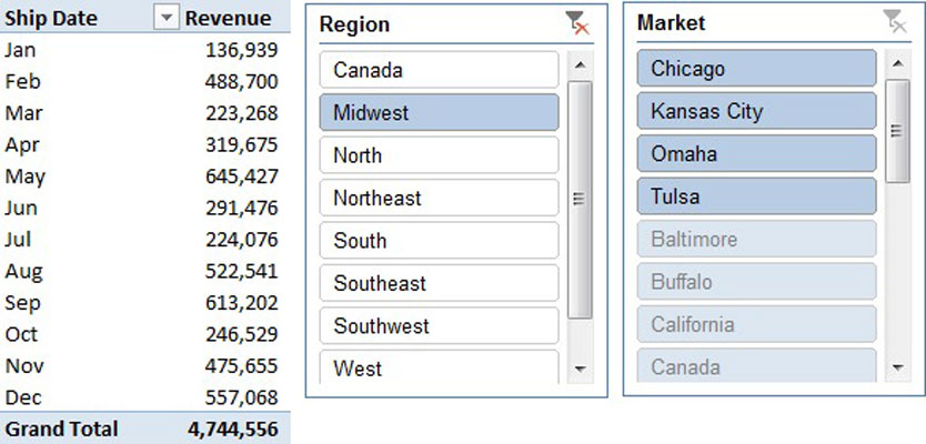
One of the more useful benefits of the slicer is that it responds to other slicers, providing a cascading filter effect. For example, the figure illustrates not only that clicking on Midwest in the Region slicer filters the pivot table but that the Market slicer also responds, by highlighting the markets that belong to the Midwest region. Microsoft calls this behavior cross-filtering.

As useful as the slicer is, it is, unfortunately, extremely bad for Power Pivot performance. Every time a slicer is changed, Power Pivot must recalculate all values and measures in the pivot table. To do that, Power Pivot must evaluate every tile in the selected slicer and process the appropriate calculations based on the selection.

Slicers tied to columns that contain lots of unique values will often cause a larger performance hit than columns containing only a handful of values. If a slicer contains a large number of tiles, consider using a Pivot Table Filter drop-down list instead.

On a similar note, be sure to right-size column data types. A column with few distinct values is lighter than a column with a high number of distinct values. If you’re storing the results of a calculation from a source database, reduce the number of digits (after the decimal) to be imported. This reduces the size of the dictionary and, possibly, the number of distinct values.

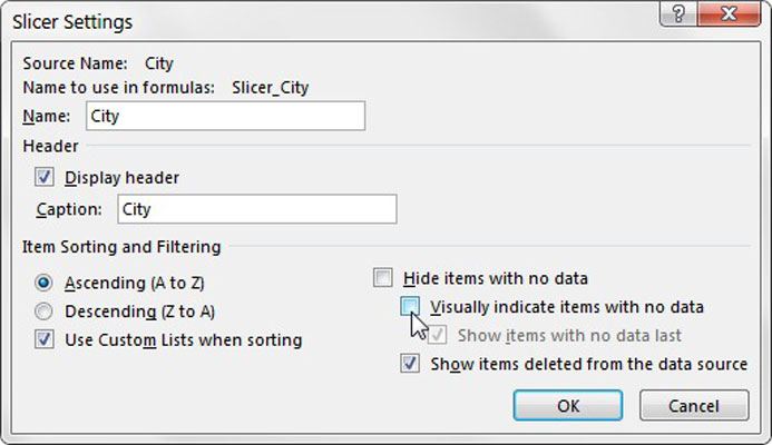
Disabling the cross-filter behavior of a slicer essentially prevents that slicer from changing selections when other slicers are clicked. This prevents the need for Power Pivot to evaluate the titles in the disabled slicer, thus reducing processing cycles. To disable the cross-filter behavior of a slicer, select Slicer Settings to open the Slicer Settings dialog box. Then simply deselect the Visually Indicate Items with No Data option.

Use calculated measures instead of calculated columns, if possible. Calculated columns are stored as imported columns. Because calculated columns inherently interact with other columns in the model, they calculate every time the pivot table updates, whether they are being used or not. Calculated measures, on the other hand, calculate only at query time.

Calculated columns resemble regular columns in that they both take up space in the model. In contrast, calculated measures are calculated on the fly and do not take space.

If you continue to run into performance issues with your Power Pivot reports, you can always buy a better PC — in this case, by upgrading to a 64-bit PC with 64-bit Excel installed.

Power Pivot loads the entire data model into RAM whenever you work with it. The more RAM your computer has, the fewer performance issues you see. The 64-bit version of Excel can access more of your PC’s RAM, ensuring that it has the system resources needed to crunch through bigger data models. In fact, Microsoft recommends 64-bit Excel for anyone working with models made up of millions of rows.

But before you hurriedly start installing 64-bit Excel, you need to answer these questions:

Do you already have 64-bit Excel installed?

Are your data models large enough?

Do you have a 64-bit operating system installed on your PC?

Will your other add-ins stop working?