


The order of operations: the fun in fundamentals
You can’t put on your sock after you put on your shoe, can you? At least, you shouldn’t! The same concept applies to mathematical operations. There’s a specific order as to which operation you perform first, second, third, and so on. At this point, it should be second nature, but because the concept is so important (especially when you start doing more complex calculations), a quick review is worth it, starting with everyone’s favorite mnemonic device.Please excuse who? Oh, yeah, you remember this one — my dear Aunt Sally! The old mnemonic still stands, even as you get into more complicated problems. Please Excuse My Dear Aunt Sally is a mnemonic for the acronym PEMDAS, which stands for
- Parentheses (including absolute value, brackets, fraction lines, and radicals)
- Exponents (and roots)
- Multiplication and Division (from left to right)
- Addition and Subtraction (from left to right)
You should also have a good grasp on the properties of equality. If you do, you’ll have an easier time simplifying expressions. Here are the properties:
- Reflexive property: a = a. For example, 4 = 4.
- Symmetric property: If a = b, then b = a. For example, if 2 + 8 = 10, then 10 = 2 + 8.
- Transitive property: If a = b and b = c, then a = c. For example, if 2 + 8 = 10 and 10 = 5 × 2, then 2 + 8 = 5 × 2.
- Commutative property of addition: a + b = b + a. For example, 3 + 4 = 4 + 3.
- Commutative property of multiplication: a × b = b × a. For example, 3 × 4 = 4 × 3.
- Associative property of addition: a + (b + c) = (a + b) + c. For example, 3 + (4 + 5) = (3 + 4) + 5.
- Associative property of multiplication: a × (b × c) = (a × b) × c. For example, 3 × (4 × 5) = (3 × 4) × 5.
- Additive identity: a + 0 = a. For example, 4 + 0 = 4.
- Multiplicative identity: a × 1 = a. For example, –18 × 1 = –18.
- Additive inverse property: a + (–a) = 0. For example, 5 + (–5) = 0.
- Multiplicative inverse property:
 , as long as
  . For example,
- Distributive property: a(b + c) = a × b + a × c. For example, 5(4 + 3) = 5 × 4 + 5 × 3.
- Multiplicative property of zero: a × 0 = 0. For example, 4 × 0 = 0.
- Zero product property: If a × b = 0, then a = 0 or b = 0. For example, if x(2x – 3) = 0, then x = 0 or (2x – 3) = 0.
How to solve equalities
Just as simplifying expressions is a basic process in pre-algebra, solving for variables is the basis of algebra. And both are essential to the more complex concepts covered in pre-calculus.Solving linear equations with the general format of ax + b = c, where a, b, and c are constants, is relatively easy using the properties of numbers. The goal, of course, is to isolate the variable, x.
One type of equation you can’t forget is the absolute value equation. The absolute value of a number is defined as its distance from 0. In other words,

Check out the following example.
Solve for x: 3(2x – 4) = x – 2(3 – 2x)
x = 6
First, using the distributive property, distribute the 3 and the –2 to get 6x – 12 = x – 6 + 4x. Then combine like terms and solve using algebra, like so: 6x – 12 = 5x –6 giving you x – 12 = –6, and, finally, x = 6.How to graph equalities and inequalities
Graphs are visual representations of mathematical equations. In pre-calculus, you’ll be introduced to many new mathematical equations and then be expected to graph them. You will have plenty of practice graphing these equations when you read the material involving the more complex equations. In the meantime, it’s important to practice the basics: graphing linear equations and inequalities.The graphs of linear equations and inequalities exist on the Cartesian coordinate system, which is made up of two axes: the horizontal, or x-axis, and the vertical, or y-axis. Each point on the coordinate plane is called a Cartesian coordinate pair and has an x coordinate and a y coordinate. The notation for any point on the coordinate plane looks like this: (x, y). A set of these ordered pairs that can be graphed on a coordinate plane is called a relation. The x values of a relation are its domain, and the y values are its range. For example, the domain of the relation R = {(2,4), (–5,3), (1,–2)} is {2,–5,1}, and the range is 4,3,–2}.
You can graph a linear equation using two points or by using the slope-intercept form. The same can be used when graphing linear inequalities. These approaches are reviewed in the following sections.How to graph with two points
To graph a line using two points, choose two numbers and plug them into the equation to solve for the range (y) values. After you plot these points (x, y) on the coordinate plane, you can draw the line through the points.A nice alternative is to use the two intercepts, the points that fall on the x- or y-axes. To find the x-intercept (x, 0), plug in 0 for y and solve for x. To find the y-intercept (0, y), plug in 0 for x and solve for y. For example, to find the intercepts of the linear equation 2x + 3y = 12, start by plugging in 0 for y: 2x + 3(0) = 12. Then, using properties of numbers, solve for x and you get x = 6. So, the x-intercept is (6, 0). For the y-intercept, plug in 0 for x and solve for y: 2(0) + 3y = 12, which gives you y = 4. Therefore, the y-intercept is (0, 4). At this point, you can plot those two points and connect them to graph the line, because, as you learned in geometry, two points make a line. See the resulting graph.
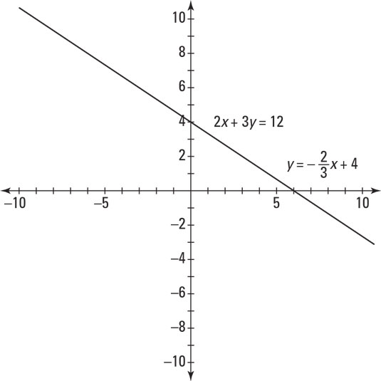 Graph of 2x + 3y = 12.
Graph by using the slope-intercept form
The slope-intercept form of a linear equation gives a great deal of helpful information in a nice package. The equation y = mx + b immediately gives you the y-intercept (b); it also gives you the slope (m). Slope is a fraction that gives you the rise over the run. To change equations that aren’t written in slope-intercept form, you simply solve for y. For example, if you use the linear equation 2x + 3y = 12, you start by subtracting 2x from each side: 3y = –2x + 12. Next, you divide all the terms by 3 giving you
Now that the equation is in slope-intercept form, you know that the y-intercept is 4, and you can plot this point on the coordinate plane. Then you can use the slope to plot a second point. From the slope-intercept equation, you know that the slope is

This tells you that the rise is –2 and the run is 3. From the point (0, 4), plot the point 2 down and 3 to the right. In other words, (3, 2). Lastly, connect the two points to graph the line. The resulting graph is identical to the figure shown.
Graphing inequalities
Similar to graphing linear equations, graphing linear inequalities begins with plotting two points. However, because inequalities are used for comparisons — greater than, less than, or equal to — you have two more questions to answer after finding two points:
- Is the line dashed (less than or greater than) or solid (less than or equal to or greater than or equal to)?
- Do you shade under the line (y is less than or y is less than or equal to) or above the line (y is greater than or y is greater than or equal to)?
How to use graphs to find distance, midpoint, and slope
Graphs are more than just pretty pictures. From a graph, it’s possible to choose two points and then figure out the distance between them, the midpoint of the segment connecting them, and the slope of the line running through them. As graphs become more complex in both pre-calculus and calculus, you’re asked to find and use all three of these pieces of information. Aren’t you lucky?Finding the distance
Distance refers to how far apart two things are. In this case, you’re finding the distance between two points. Knowing how to calculate distance is helpful for when you get to conics. To find the distance between two points (x1,n y1) and (x2,n y2), use the following formula:
Calculating the midpoint
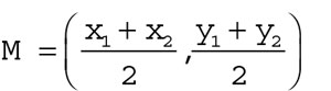
The midpoint is the middle of a segment. This concept also comes up in conics and is ever so useful for all sorts of other pre-calculus calculations. To find the coordinates of the midpoint, M, of the points (x1,n y1) and (x2,n y2), you just need to average the x and y values and express them as an ordered pair, like so:
Discovering the slope
Slope is a key concept for linear equations, but it also has applications for trigonometric functions and is essential for differential calculus. Slope describes the steepness of a line on the coordinate plane (think of a ski slope). Use this formula to find the slope, m, of the line (or segment) connecting the two points (x1,n y1) and (x2,n y2):
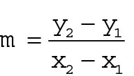
Note: Positive slopes move upward as you move from left to right. Negative slopes move downward as you move from left to right. Horizontal lines have a slope of 0, and vertical lines have an undefined slope.
