


Fields like engineering, electricity, and quantum physics all use imaginary numbers in their everyday applications. An imaginary number is basically the square root of a negative number. The imaginary unit, denoted i, is the solution to the equation i2 = –1.
A complex number can be represented in the form a + bi, where a and b are real numbers and i denotes the imaginary unit. In the complex number a + bi, a is called the real part and b is called the imaginary part. Real numbers can be considered a subset of the complex numbers that have the form a + 0i. When a is zero, then 0 + bi is written as simply bi and is called a pure imaginary number.
How to perform operations with and graph complex numbers
Complex numbers in the form a + bi can be graphed on a complex coordinate plane. Each complex number corresponds to a point (a, b) in the complex plane. The real axis is the line in the complex plane consisting of the numbers that have a zero imaginary part: a + 0i. Every real number graphs to a unique point on the real axis. The imaginary axis is the line in the complex plane consisting of the numbers that have a zero real part:0 + bi. The figure shows several examples of points on the complex plane.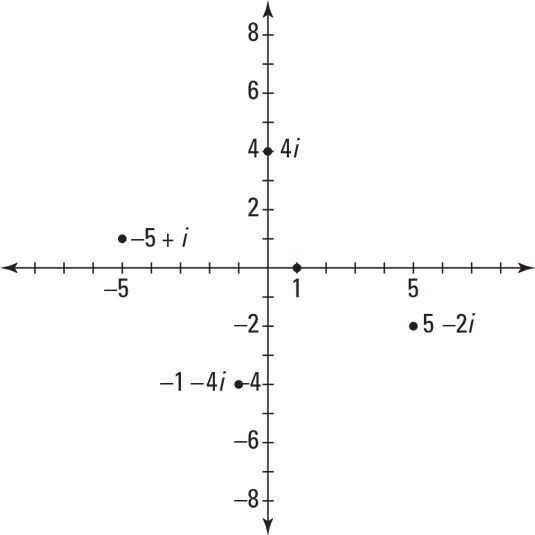 Graphing complex numbers.
Adding and subtracting complex numbers is just another example of collecting like terms: You can add or subtract only real numbers, and you can add or subtract only imaginary numbers.
When multiplying complex numbers, you FOIL the two binomials. All you have to do is remember that the imaginary unit is defined such that i2 = –1, so any time you see i2 in an expression, replace it with –1. When dealing with other powers of i, notice the pattern here:
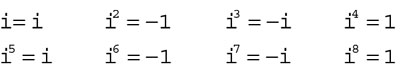
This continues in this manner forever, repeating in a cycle every fourth power. To find a larger power of i, rather than counting forever, realize that the pattern repeats. For example, to find i243, divide 4 into 243 and you get 60 with a remainder of 3. The pattern will repeat 60 times and then you’ll have 3 left over, so i243 = i240 × i3 = 1 × i3, which is –i.
The conjugate of a complex number a + bi is a – bi, and vice versa. When you multiply two complex numbers that are conjugates of each other, you end up with a pure real number:
(a + bi)(a – bi) = a2 – abi + abi – b2i2
Combining like terms and replacing i2 with –1: = a2 – b2(–1) = a2 + b2
Remember that absolute value bars enclosing a real number represent distance. In the case of a complex number, |a + bi| represents the distance from the point to the origin. This distance is always the same as the length of the hypotenuse of the right triangle drawn when connecting the point to the x- and y-axes.
When dividing complex numbers, you multiply numerator and denominator by the conjugate. If the square root of a number is involved, then you’ll be rationalizing the denominator.
In general, a division problem involving complex numbers looks like this:
![]()
Round a pole: how to graph polar coordinates
Up until now, your graphing experiences may have been limited to the rectangular coordinate system. The rectangular coordinate system gets that name because it’s based on two number lines perpendicular to each other. It’s now time to take that concept further and introduce polar coordinates.In polar coordinates, every point is located around a central point, called the pole, and is named (r,nθ). r is the radius, and θ is the angle formed between the polar axis (think of it as what used to be the positive x-axis) and the segment connecting the point to the pole (what used to be the origin).
In polar coordinates, angles are labeled in either degrees or radians (or both). The figure shows the polar coordinate plane.
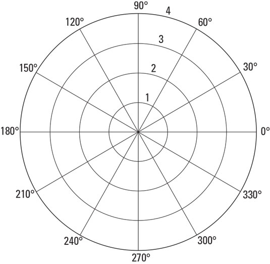 Graphing round and round on the polar coordinate plane.
Notice that a point on the polar coordinate plane can have more than one name. Because you’re moving in a circle, you can always add or subtract 2π to any angle and end up at the same point. This is an important concept when graphing equations in polar forms, so this discussion will cover it well.
When both the radius and the angle are positive, the angle moves in a counterclockwise direction. If the radius is positive and the angle is negative, the point moves in a clockwise direction. If the radius is negative and the angle is positive, find the point where both are positive first and then reflect that point across the pole. If both the radius and the angle are negative, find the point where the radius is positive and the angle is negative and then reflect that across the pole.
Changing to and from polar
You can use both polar and rectangular coordinates to name the same point on the coordinate plane. Sometimes it’s easier to write an equation in one form than the other, so this should familiarize you with the choices and how to switch from one to another. This figure shows how to determine the relationship between these two not-so-different methods.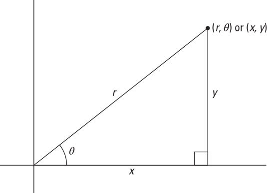 A right triangle reveals the relationship between rectangular and polar coordinates.
Some right triangle trigonometry and the Pythagorean Theorem:


x2 + y2 = r2
Graphing Polar Equations
When given an equation in polar format and asked to graph it, you can always go with the plug-and-chug method: Pick values for θ from the unit circle that you know so well and find the corresponding value of r. Polar equations have various types of graphs, and it’s easier to graph them if you have a general idea what they look like.Archimedean spiral
r = aθ gives a graph that forms a spiral. a is a constant that’s multiplying the angle. If a is positive, the spiral moves in a counterclockwise direction, just like positive angles do. If a is negative, the spiral moves in a clockwise direction.Cardioid
You may recognize the word cardioid if you’ve ever worked out and done your cardio. The word relates to the heart, and when you graph a cardioid, it does look like a heart, of sorts. Cardioids are written in the form OR
OR  .
.
The cosine equations are hearts that point to the left or right, and the sine equations open up or down.
Rose
A rose by any other name is … a polar equation. If r = asinbθ or r = acosbθ, the graphs look like flowers with petals. The number of petals is determined by b. If b is odd, then there are b (the same number of) petals. If b is even, there are 2b petals.Circle
When r = asinθ or r = acosθ, you end up with a circle with a diameter of a. Circles with cosine in them are centered on the x-axis, and circles with sine in them are centered on the y-axis. These are particular types of circles passing through the origin.Lemniscate
A lemniscate makes a figure eight; that’s the best way to remember it.![]() forms a figure eight between the axes, and
forms a figure eight between the axes, and
![]() forms a figure eight that lies on one of the axes as a line of symmetry.
forms a figure eight that lies on one of the axes as a line of symmetry.
Limaçon
A cardioid is really a special type of limaçon, which is why they look similar to each other when you graph them. The familiar forms of limaçons are![]() OR
OR ![]()


