


The Breusch-Pagan (BP) test is one of the most common tests for heteroskedasticity. It begins by allowing the heteroskedasticity process to be a function of one or more of your independent variables, and it’s usually applied by assuming that heteroskedasticity may be a linear function of all the independent variables in the model. This assumption can be expressed as
The values for
aren’t known in practice, so the
are calculated from the residuals and used as proxies for
Generally, the BP test is based on the estimation of
Alternatively, a BP test can be performed by estimating
Here’s how to perform a BP test:
Estimate your model using OLS:

Obtain the predicted Y values after estimating the model.
Estimate the auxiliary regression using OLS:

From this auxiliary regression, retain the R-squared value:

Calculate the F-statistic or the chi-squared statistic:

The degrees of freedom for the F-test are equal to 1 in the numerator and n – 2 in the denominator. The degrees of freedom for the chi-squared test are equal to 1. If either of these test statistics is significant, then you have evidence of heteroskedasticity. If not, you fail to reject the null hypothesis of homoskedasticity.
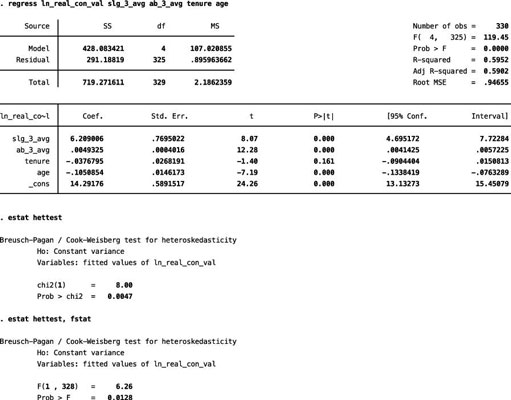
To see how the BP test works, use some data about Major League Baseball players. First, estimate a model with the natural log of the player’s contract value as the dependent variable and several player characteristics as independent variables, including three-year averages for the player’s slugging percentage and at-bats, the player’s age, and the player’s tenure with the current team.
Then run the BP test in STATA, which retains the predicted Y values, estimates the auxiliary regression internally, and reports the chi-squared test. You can also request that STATA conduct the F-test version of the test.
Both results are shown in the figure, and they’re consistent in rejecting the null hypothesis of homoskedasticity. Therefore, the statistical evidence implies that heteroskedasticity is present.
A weakness of the BP test is that it assumes the heteroskedasticity is a linear function of the independent variables. Failing to find evidence of heteroskedasticity with the BP doesn’t rule out a nonlinear relationship between the independent variable(s) and the error variance. Additionally, the BP test isn’t useful for determining how to correct or adjust the model for heteroskedasticity.
