Distribution is the statistical term that describes the relative likelihood of observing values for a variable factor. When you think of a Six Sigma initiative and the critical performance characteristics of a product or service — either output Ys or input Xs — you should begin thinking of them as distributions. Variation is inherent in all Xs and Ys, so you will see distributions in your measurements.
In 1891, the famous scientist Lord Kelvin provided valuable insight for future Six Sigma practitioners:
When you can measure what you are speaking about, and express it in numbers, you know something about it; but when you cannot express it in numbers, your knowledge is of a meager and unsatisfactory kind. It may be the beginning of knowledge, but you have scarcely, in your thoughts, advanced to the state of science.
In other words, if you want to make big performance gains, you need to harness the power of statistics and data analysis to take you out of the realm of intuition and estimation and into the realm of objective truth. Statistics — and its embodiment in Six Sigma — is like vegetables: It’s not always what you want to have, but you know it’s good for you.
Statistics is the branch of mathematics that distills raw numbers, data, and measurements into knowledge and insight. If you understand a little bit about statistics, you can create a data-leveraging environment that you can use to understand or improve something.
You don’t have to have a PhD in statistics to be a Six Sigma practitioner, but you should have a grasp of statistical concepts. Armed with two quantities — a measure of location and a measure of spread — you can describe any type of distribution in scientific terms. Lord Kelvin would be proud!
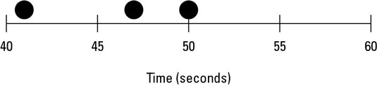
Suppose you need to find out how long filling out a certain purchase order form takes. Each time you fill out the form, you record the elapsed time to the nearest second and plot the result as a dot along a horizontal time scale. You can see the first three times you fill out the form, with times of 41, 50, and 47 seconds.
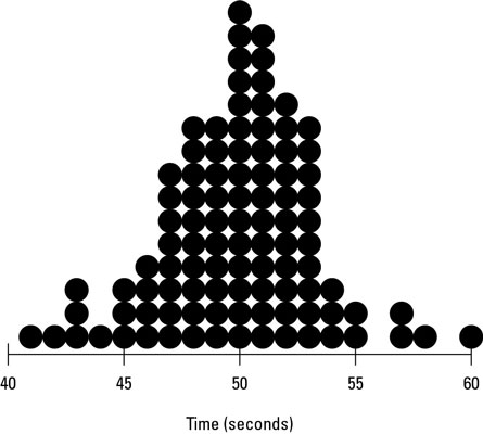
See how your data reveals that variation is inherent in the process? Continuing the study, you take a total of 100 purchase order time measurements. Whenever you encounter a measurement that already has a recording (such as 47 seconds), you simply stack another dot on top of the previous dot.
Notice that the output values that occur often pile up with multiple dots. For example, 50 seconds is the purchase order completion time that occurs more frequently than any other. Consequently, it has the highest peak in the chart (15 occurrences). Output values that happen less frequently have lower heights, and output values that were never observed have no dots at all.
You can see how the measured output is distributed along its scale of measure: time. Looking at the chart, you can predict that if you were to measure another cycle of the purchase order process, the elapsed time would most likely be around 50 seconds. A completion time of 30 seconds or 80 seconds, for example, is just not likely to happen.