


Microsoft's continually enhancing the computing power of the Excel worksheet through the addition of new built-in functions and formulas. Microsoft Excel 2016 now contains some new Text and Logical functions, such as IFS, SWITCH and TEXTJOIN functions, that you definitely will want to check out. Regarding formula updates, discover how easy it is to create simple formulas in excel for returning specific information from worksheet cells identified with the new Stocks or Geography data type.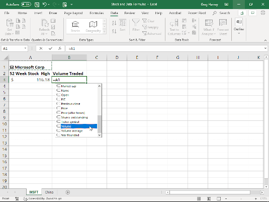 Creating a formula that retrieves MSFT volume traded.
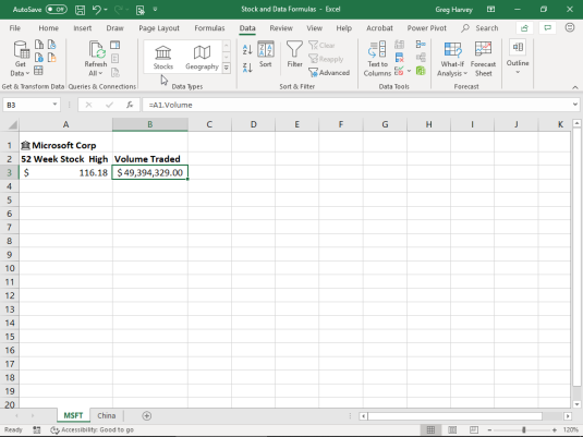 MSFT worksheet with the result of the MSFT volume traded formula.
 Creating a formula that returns China’s CPI.
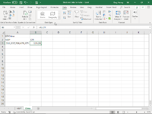 China worksheet with formula that returns the CPI.
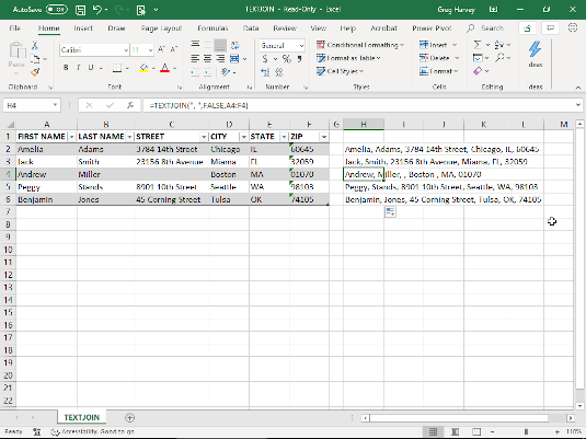 Using TEXTJOIN to combine text entries in an Excel table.
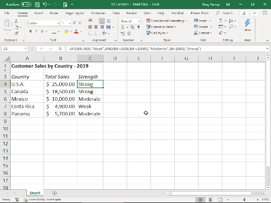 Using the IFS function to evaluate three conditions: Weak, Moderate, or Strong.
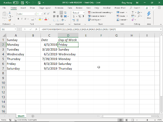 Using the SWITCH function to swap out the number returned by the WEEKDAY function with its name.
Creating a formula that retrieves MSFT volume traded. MSFT worksheet with the result of the MSFT volume traded formula.Formulas with the Stocks data type
The new Stocks data type in Excel 2016 enables you to retrieve and insert all types of financial information about a stock in succeeding cells in the same row, using the Show Card or Insert Data buttons. You can also build simple formulas that return this financial information anywhere in the worksheet. Figures 2-1 and 2-2 in the Formula Updates gallery above illustrate how you do this. In Fig. 2-1, using the Stocks data type, cell A1 of the worksheet that originally contained the label, MSFT, has been associated with Microsoft Corp. In cell B3, I am building a formula that returns the volume traded of Microsoft stock:- With the cell cursor in cell B3, type = (equal) and then click cell A1 containing the Microsoft Corp Stocks data.
- Scroll down the drop-down menu that appears beneath cell B3 containing the list of various financial data the formula can return until Volume is selected.
- Double-click Volume in the drop-down menu to insert it into the formula so that the formula now reads, =A1.Volume.
- Click the Enter button on the Formula bar to close the drop-down menu and complete the formula entry in cell B3.
Creating a formula that returns China’s CPI. China worksheet with formula that returns the CPI.Formulas with the Geography data type
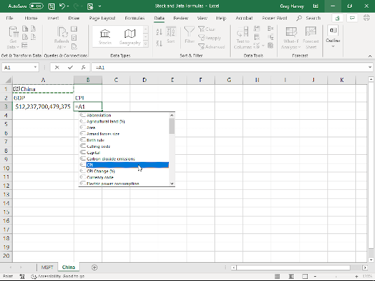
Figures 2-3 and 2-4 in the Formula Updates gallery above illustrate how easy it is to build formulas using cells associated with the new Geography data type. In Fig. 2-3, the label, China, entered into cell A1 has been associated with the People's Republic of China using the Geography data type. In cell B3, you can create a formula that returns the CPI (Consumer Price Index) as follows:- With the cell cursor in cell B3, type = (equal) and then click cell A1 containing the China Geography data.
- Double-click CPI in the drop-down menu that appears to insert CPI into the formula so that now reads, =A1.CPI, on the Formula bar.
- Click the Enter button on the Formula bar to close the drop-down menu and insert the formula into cell B3.
T(Value)
The T function checks whether or not the Value argument is or refers to a text entry. If true, the function returns the value. If false, the function returns "" empty text. Note that Excel automatically evaluates whether any entry you make in the worksheet is text or a value. The T function goes a step further by bringing the entry forward to a new cell only when it's evaluated as text. Using TEXTJOIN to combine text entries in an Excel table.TEXTJOIN(delimiter,ignore_empty,text1,...)
The TEXTJOIN function concatenates (combines) the text entries from multiple cell ranges as specified by the text1, ... argument(s) using the character (enclosed in quotes) specified as the delimiter argument. If no delimiter argument is specified, Excel concatenates the text as though you had use the & operator. The ignore_empty logical argument specifies whether or not to ignore empty cells in the text1, ... arguments. If no ignore_empty argument is specified, Excel ignores empty cells as though you had entered TRUE. Fig. 2-5 in the Function Updates gallery above illustrates the use of this function to combine the text entries made in the Excel table in cell range A2:F6 in the cell range, H. The original formula entered into cell H2:H6. The original formula entered into cell H2 reads:=TEXTJOIN(", ",FALSE,A2:F2)
This formula specifies the , (comma) followed by a space as the delimiter separating the text entries combined from the cell range A2:F2. Note that because the ignore_empty argument is set to FALSE in the original formula when it's copied down column H to include all four rows of the Excel table, the formula in cell H4 shows that the Street entry in cell C4 of the Excel table is missing with the , , string between Miller and Boston.
Using the IFS function to evaluate three conditions: Weak, Moderate, or Strong.IFS(logical_test1.value_if_TRUE1,logical_test2,value_if_TRUE2,...)
The IFS logical function tests whether or not one or more logical_test arguments are TRUE or FALSE. If any found TRUE, Excel returns the corresponding value argument. This function is great as it eliminates the need for multiple nested IF functions in a formula when testing for more than a single TRUE or FALSE outcome. Fig. 2-6 in the Function Updates gallery above illustrates how this works. The formula entered into cell C4 with the IFS function tests for one of three conditions in cell B4:- If the value is less than 5,000, the formula returns the label, Weak.
- If the value is between 5,000 and 10,000, the formula returns the label, Moderate.
- If the value is more than 5,000, the formula returns the label, Strong.
Using the SWITCH function to swap out the number returned by the WEEKDAY function with its name.


