


When charting a bunch of values, Excel 2013 isn’t too careful how it formats the values that appear on the y-axis. If you’re not happy with the way the values appear on either the x-axis or y-axis, you can easily change the formatting as follows:
Click the x-axis or y-axis directly in the chart and then click Horizontal Axis or Vertical Axis on its drop-down list.
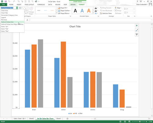
Excel surrounds the axis you select with selection handles.
Click the Format Selection button in the Current Selection group of the Format tab.
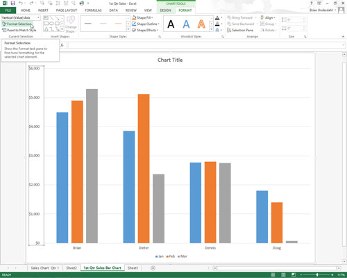
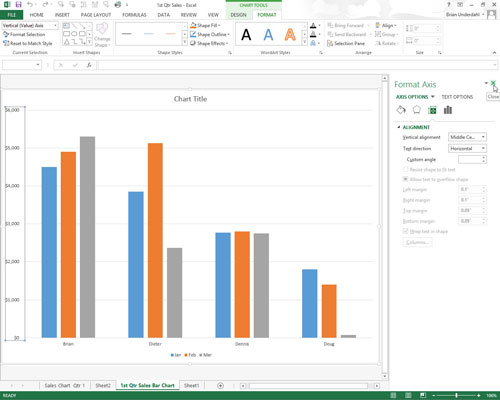
Excel opens the Format Axis task pane with Axis Options under the Axis Options group selected.
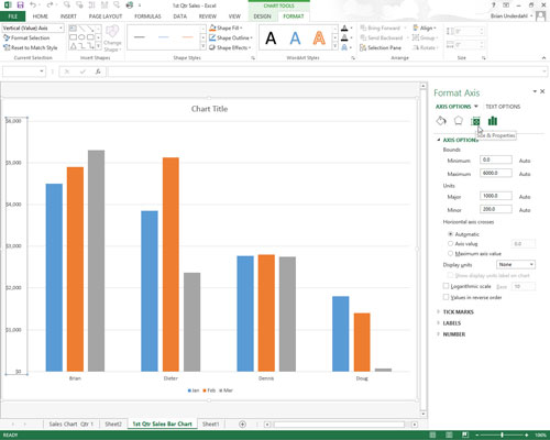
To change the scale of the axis, the appearance of its tick marks, and where it crosses the other axis, change the appropriate options under Axis Options as needed.

These options include those that fix the maximum and minimum amount for the first and last tick mark on the axis, display the values in reverse order, and apply a logarithmic scale. You can display units on the axis and divide the values by those units, reposition the tick marks on the axis, and modify the value at which the other axis crosses.
To change the number formatting for all values on the selected axis, click the Number option.
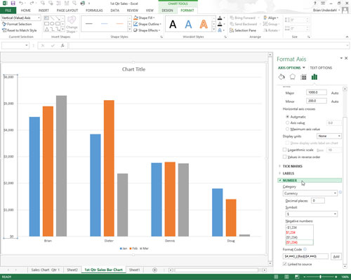
Then select the number format you want to apply in the Category drop-down list box followed by the appropriate options associated with that format. To assign the same number formatting to the values on the selected axis as assigned to the values in their worksheet cells, select the Linked To Source check box.
To change the alignment and orientation of the labels on the selected axis, click the Size & Properties button under Axis Options on the Format Axis task pane.
Then, indicate the new orientation by clicking the desired vertical alignment in the Vertical Alignment drop-down list box and desired text direction in the Text Direction drop-down list.
To change the default font, font size, or other text attributes for entries along the selected x- or y-axis, click the appropriate command buttons in the Font group on the Home tab.
Click the Close button to close the Format Axis task pane.
As you choose new options for the selected axis, Excel 2013 shows you the change in the chart. However, these changes are set in the chart only when you click Close in the Format Axis dialog box.


