


Excel 2016's Filter feature makes it a breeze to hide everything in a data list except the records you want to see. To filter the data list to just those records that contain a particular value, you then click the appropriate field's AutoFilter button to display a drop-down list containing all the entries made in that field and select the one you want to use as a filter.
Excel then displays only those records that contain the value you selected in that field. (All other records are hidden temporarily.)
If the column headings of your data list table don't currently have filter drop-down buttons displayed in their cells after the field names, you can add them simply by clicking Home→Sort & Filter→Filter or pressing Alt+HSF.
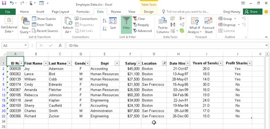
For example, in the figure, I filtered the Employee Data List to display only those records in which the Location is either Boston or San Francisco by clicking the Location field's AutoFilter button and then clicking the (Select All) check box to remove its check mark. I then clicked the Boston and San Francisco check boxes to add check marks to them before clicking OK. (It's as simple as that.)
After you filter a data list so that only the records you want to work with are displayed, you can copy those records to another part of the worksheet to the right of the database (or better yet, another worksheet in the workbook). Simply select the cells, then click the Copy button on the Home tab or press Ctrl+C, move the cell cursor to the first cell where the copied records are to appear, and then press Enter. After copying the filtered records, you can then redisplay all the records in the database or apply a slightly different filter.
If you find that filtering the data list by selecting a single value in a field drop-down list box gives you more records than you really want to contend with, you can further filter the database by selecting another value in a second field's drop-down list. For example, suppose that you select Boston as the filter value in the Location field's drop-down list and end up with hundreds of Boston records displayed in the worksheet.
To reduce the number of Boston records to a more manageable number, you could then select a value (such as Human Resources) in the Dept field's drop-down list to further filter the database and reduce the records you have to work with onscreen. When you finish working with the Boston Human Resources employee records, you can display another set by displaying the Dept field's drop-down list again and changing the filter value from Human Resources to some other department, such as Accounting.
When you're ready to display all the records in the database again, click the filtered field's AutoFilter button (indicated by the appearance of a cone filter on its drop-down button) and then click the Clear Filter from (followed by the name of the field in parentheses) option near the middle of its drop-down list.
You can temporarily remove the AutoFilter buttons from the cells in the top row of the data list containing the field names and later redisplay them by clicking the Filter button on the Data tab or by pressing Alt+AT or Ctrl+Shift+L.


