


Use the Custom AutoFilter dialog box in Excel 2010 to locate records that either match all criteria or meet one or the other criteria. You can use this method when you want to filter data based on a range of values (for example, you can filter for values that are greater than or equal to 1,000 in a specified column).
Excel 2010 tables automatically display filter arrows beside each of the column headings. To display the filter arrows so that you can filter data, format a range as a table using the Table button on the Insert tab. Or, you can click the Filter button in the Sort & Filter group on the Data tab.
Click the filter arrow for the numeric column by which you want to filter data.
A drop-down list of filter options appears.

Select a number filter.
The Custom AutoFilter dialog box appears.
In the first list box on the right, type the value you want to filter.
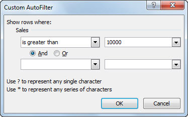
You also can choose any item displayed in the drop-down list.
(Optional) To choose additional criteria, select And or Or; then specify the data for the second criteria.
Choosing “And” means that both criteria must be met; choosing “Or” means that either criteria can be met.
Click OK.
The filtered records display in the worksheet.


