


It’s always a good idea to use range names in worksheets for all the previous versions of Excel designed for desktop and laptop computers. With this new version of Excel designed for touchscreen devices, such as Windows 10 tablets and smartphones, as well, it’s easy to become a fanatic about their use. You can save yourself oodles of time and tons of frustration by locating and selecting the data tables and lists in your worksheets on these touch devices via range names. Contrast simply tapping their range names on Excel’s Name box’s drop-down list to go to and select them to having first to swipe and swipe to locate and display their cells before dragging through their cells with your finger or stylus.
How to name Excel ranges and cells
When assigning Excel range names to a cell or cell range, you need to follow a few guidelines:- Range names must begin with a letter of the alphabet, not a number.
For example, instead of 01Profit, use Profit01.
- Range names cannot contain spaces.Instead of a space, use the underscore (Shift+hyphen) to tie the parts of th
e name together. For example, instead of Profit 01, use Profit_01.
- Range names cannot correspond to cell coordinates in the worksheet.
For example, you can’t name a cell Q1 because this is a valid cell coordinate. Instead, use something like Q1_sales.
- Range names must be unique within their scope.
That is, all of the Excel worksheets in the workbook when the scope is set to Workbook (as it is by default) or just a specific sheet in the workbook when the scope is set to a particular worksheet, such as Sheet1 or Income Analysis (when the sheet is named).
- Select the single cell or range of cells that you want to name.
- Click Formulas → Defined Names → Define Name (Alt+MZND) to open the New Name dialog box.
 Naming a cell range in the Excel worksheet in the New Name dialog box.
 - Type the name for the selected cell or cell range in the Name Box.
- (Optional) To limit the scope of the Excel range name to a particular worksheet rather than the entire workbook (the default), click the drop-down button in the Scope drop-down list box and then click the name of sheet to which the range is to be restricted.
- (Optional) To add a comment describing the function and/or extent of the range name, click the Comment text box and then type your comments.
- Check the cell range that the new range name will encompass in the Refers to text box and make an adjustment, if necessary.
If this cell range is not correct, click the Collapse button (the up arrow button) to the right of the Refers To text box to condense the New Dialog box to the Refers To text box and then click the appropriate cell or drag through the appropriate range before you click Expand button (the down arrow to the right of the text box) to restore the New Name dialog box to its normal size.
- Click the OK button to complete the definition of the range name and to close the New Range name dialog box. To quickly name a cell or cell range in an Excel worksheet from the Name Box on the Formula bar, follow these steps:
- Select the single cell or range of cells that you want to name.
- Click the cell address for the current cell that appears in the Name Box on the far left of the Formula bar.
Excel selects the cell address in the Name Box.
- Type the name for the selected cell or cell range in the Name Box.
When typing the range name, you must follow Excel’s naming conventions listed above.
- Press Enter.
You can also accomplish the same thing in Excel by selecting Home → Find & Select (with the binoculars icon) → Go To or by pressing F5 or Ctrl+G to open the Go To dialog box. Double-click the desired range name in the Go To list box (alternatively, select the name followed by OK). Excel moves the cell cursor directly to the named cell. If you select a cell range, all the cells in that range are selected as well.
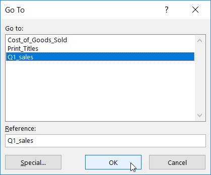 Select the named cell range to go to in an Excel workbook.
Naming cells to identify Excel range formulas
Cell names are not only a great way to identify and find cells and cell ranges in your spreadsheet, but they’re also a great way to make out the purpose of your formulas. For example, suppose that you have a simple formula in cell K3 that calculates the total due to you by multiplying the hours you work for a client (in cell I3) by the client’s hourly rate (in cell J3). Normally, you would enter this formula in cell K3 as=I3*J3
However, if you assign the name Hours to cell I3 and the name Rate to cell J3, in cell K3 you could enter the formula
=Hours*Rate
It’s doubtful that anyone would dispute that the function of the formula =Hours*Rate is much easier to understand than =I3*J3.
To enter an Excel formula using cell names rather than cell references, follow these steps:
- Assign range names to the individual cells.For this example, give the name Hours to cell I3 and the name Rate to cell J3.
- Place the cell cursor in the cell where the formula is to appear. For this example, put the cell cursor in cell K3.
- Type = (equal sign) to start the formula.
- Select the first cell referenced in the formula by selecting its cell (either by clicking the cell or moving the cell cursor into it).For this example, you select the Hours cell by selecting cell I3.
- Type the arithmetic operator to use in the formula.For this example, you would type * (asterisk) for multiplication.
- Select the second cell referenced in the formula by selecting its cell (either by clicking the cell or moving the cell cursor into it).For this example, you select the Rate cell by selecting cell J3.
- Click the Enter button or press Enter to complete the formula.
In this example, Excel enters the formula =Hours*Rate in cell K3.
You can’t use the fill handle to copy a formula that uses cell names, rather than cell addresses, to other cells in a column or row that perform the same function. When you copy an original formula that uses names rather than addresses, Excel copies the original formula without adjusting the cell references to the new rows and columns.
Having trouble with your Excel formula? Find out how to decipher error values in an Excel formula.
Naming constants in Excel ranges
Certain formulas use constant values, such as an 8.25% tax rate or a 10% discount rate. If you don’t want to have to enter these constants into a cell of the worksheet in order to use the formulas, you create range names that hold their values and then use their range names in the formulas you create.For example, to create a constant in Excel called tax_rate (of 8.25%), follow these steps:
- Click the Define Name button on the Ribbon’s Formulas tab or press Alt+MMD to open the New Name dialog box.
- In the New Name dialog box, type the range name (tax_rate in this example) into the Name text box.Be sure to adhere to the cell range naming conventions when entering this new name.
- (Optional) To limit the scope of range name defined to just a particular worksheet instead of the entire workbook, click the name of the sheet on the Scope drop-down list.
Normally, you’re safer sticking with the default selection of Workbook as the Scope option so that you can use your constant in a formula on any of its sheets. Only change the scope to a particular worksheet when you want to use the same range name on multiple sheets of the workbook or you’re sure that you’ll use it only in formulas on that worksheet.
- Click in the Refers To text box after the equal to sign (=) and replace (enter) the current cell address with the constant value (8.25% in this example) or a formula that calculates the constant.
- Click OK to close the New Name dialog box.
- Type the range name to which you assign the constant at the place in the formula where its value is required.
- Click the Use in Formula command button on the Formulas tab (or press Alt+MS) and then click the constant’s range name on the drop-down menu that appears.
When you copy a formula that uses a range name containing a constant, its values remain unchanged in all copies of the formula that you create with the fill handle. (In other words, range names in formulas act like absolute cell addresses in copied formulas.)
Also, when you update the constant by changing its value in the Edit Name dialog box — opened by clicking the range name in the Name Manager dialog box (Alt+MN) and then clicking its Edit button — all the formulas that use that constant (by referring to the range name) are automatically updated (recalculated) to reflect this change.


