Directly Feed Excel's Internal Data Model

Imagine that you have the Transactions table you see here, and on another worksheet you have an Employees table that contains information about the employees.

This table shows transactions by employee number.

This table provides information on employees: first name, last name, and job title.

You need to create an analysis that shows sales by job title. This would normally be difficult given the fact that sales and job title are in two separate tables. But with the Internal Data Model, you can follow these simple steps:

1. Click inside the Transactions data table and start a new pivot table by choosing Insert ➪ Pivot Table from the Ribbon.
2. In the Create PivotTable dialog box, select the Add This Data to the Data Model option.

   

   When you create a new pivot table from the Transactions table, be sure to select Add This Data to the Data Model.

3. Click inside the Employees data table and start a new pivot table. Again, be sure to select the Add This Data to the Data Model option, as shown. Notice that the Create PivotTable dialog boxes are referencing named ranges. That is to say, each table was given a specific name. When you're adding data to the Internal Data Model, it's a best practice to name the data tables. This way, you can easily recognize your tables in the Internal Data Model. If you don't name your tables, the Internal Data Model shows them as Range1, Range2, and so on.
   Create a new pivot table from the Employees table, and select Add This Data to the Data Model.
4. To give the data table a name, simply highlight all data in the table, and then select Formulas→Define Name command from the Ribbon. In the dialog box, enter a name for the table. Repeat for all other tables.
5. After both tables have been added to the Internal Data Model, open the PivotTable Fields list and choose the ALL selector. This step shows both ranges in the field list.
   

   Select ALL in the PivotTable Fields list to see both tables in the Internal Data Model.
6. Build out the pivot table as normal. In this case, Job_Title is placed in the Row area, and Sales_Amount goes to the Values area. As you can see here, Excel immediately recognizes that you're using two tables from the Internal Data Model and prompts you to create a relationship between them. You have the option to let Excel autodetect the relationships between your tables or to click the Create button. Always create the relationships yourself, to avoid any possibility of Excel getting it wrong.
   

   When Excel prompts you, choose to create the relationship between the two tables.
7. Click the Create button. Excel opens the Create Relationship dialog box, shown here. There, you select the tables and fields that define the relationship. You can see that the Transactions table has a Sales_Rep field. It's related to the Employees table via the Employee_Number field.

Build the appropriate relationship using the Table and Column drop-down lists.

After you create the relationship, you have a single pivot table that effectively uses data from both tables to create the analysis you need. The following figure illustrates that, by using the Excel Internal Data Model, you've achieved the goal of showing sales by job title.

You've achieved your goal of showing sales by job title.

You see that the lower-right drop-down is named Related Column (Primary). The term primary means that the Internal Data Model uses this field from the associated table as the primary key.

The Employees table must have all unique values in the Employee_Number field, with no blanks or null values. This is the only way that Excel can ensure data integrity when joining multiple tables.

After you assign tables to the Internal Data Model, you might need to adjust the relationships between the tables. To make changes to the relationships in an Internal Data Model, click the Data tab on the Ribbon and select the Relationships command. The Manage Relationships dialog box, shown here, opens.

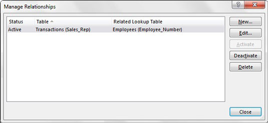The Manage Relationships dialog box enables you to make changes to the relationships in the Internal Data Model.

Here, you'll find the following commands:

• New: Create a new relationship between two tables in the Internal Data Model.
• Edit: Alter the selected relationship.
• Activate: Enforce the selected relationship, telling Excel to consider the relationship when aggregating and analyzing the data in the Internal Data Model.
• Deactivate: Turn off the selected relationship, telling Excel to ignore the relationship when aggregating and analyzing the data in the Internal Data Model.
• Delete: Remove the selected relationship.