


The Data Analysis collection of tools in Excel includes an option for calculating rank and percentile information for values in your data set. Suppose, for example, that you want to rank the sales revenue information in this worksheet. To calculate rank and percentile statistics for your data set, take the following steps.
Open the worksheet you wish to use.
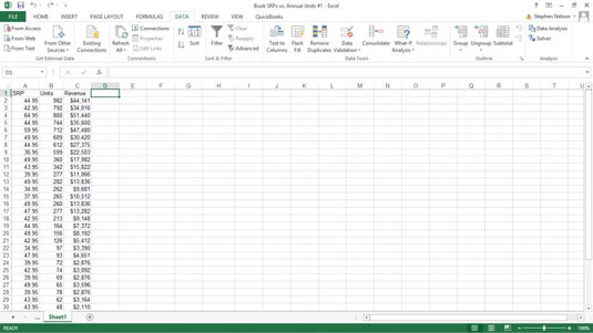
For example, a book sales information worksheet like you see here.
Begin to calculate ranks and percentiles by clicking the Data tab’s Data Analysis command button.
The Data Analysis dialog box will appear.
When Excel displays the Data Analysis dialog box, select Rank and Percentile from the list and click OK.
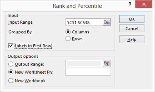
Excel displays the Rank and Percentile dialog box.
Identify the data set.
Enter the worksheet range that holds the data into the Input Range text box of the Ranks and Percentile dialog box.
To indicate how you have arranged data, select one of the two Grouped By radio buttons: Columns or Rows. To indicate whether the first cell in the input range is a label, select or deselect the Labels In First Row check box.
Describe how Excel should output the data.
Select one of the three Output Options radio buttons to specify where Excel should place the rank and percentile information.
After you select an output option, click OK.
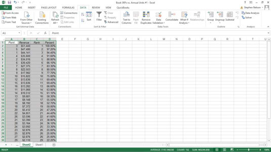
Excel creates a ranking.
