


It’s not uncommon to have reporting that joins text with numbers. For example, you may be required to show a line in your report that summarizes a salesperson’s results, like this:
John Hutchison: $5,000
The problem is that when you join numbers in a text string, the number formatting does not follow. Take a look at the figure as an example. Note how the numbers in the joined strings (column E) do not adopt the formatting from the source cells (column C).

To solve this problem, you have to wrap the cell reference for your number value in the TEXT function. Using the TEXT function, you can apply the needed formatting on the fly. The formula shown here resolves the issue:
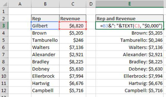
=B3&": "&TEXT(C3, "$0,000")
The TEXT function requires two arguments: a value, and a valid Excel format. You can apply any formatting you want to a number as long as it’s a format that Excel recognizes.
For example, you can enter this formula into Excel to display $99:
=TEXT(99.21,"$#,###")
You can enter this formula into Excel to display 9921%:
=TEXT(99.21,"0%")
You can enter this formula into Excel to display 99.2:
=TEXT(99.21,"0.0")
An easy way to get the syntax for a particular number format is to look at the Number Format dialog box. To see that dialog box and get the syntax, follow these steps:
Right-click any cell and select Format Cell.
On the Number format tab, select the formatting you need.
Select Custom from the Category list on the left of the Number Format dialog box.
Copy the syntax found in the Type input box.
