


 You want to use Power Pivot to analyze the data in the Customers, InvoiceHeader, and InvoiceDetails worksheets.
You can find the sample files for this exercise on in the workbook named Chapter 2 Samples.xlsx.
At this point, Power Pivot knows that you have three tables in the data model but has no idea how the tables relate to one another. You connect these tables by defining relationships between the Customers, Invoice Details, and Invoice Header tables. You can do so directly within the Power Pivot window.
If you've inadvertently closed the Power Pivot window, you can easily reopen it by clicking the Manage command button on the Power Pivot Ribbon tab.
Follow these steps to create relationships between your tables:- Activate the Power Pivot window and click the Diagram View command button on the Home tab.
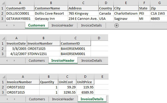
The Power Pivot screen you see shows a visual representation of all tables in the data model, as shown.
You can move the tables in Diagram view by simply clicking and dragging them. The idea is to identify the primary index keys in each table and connect them. In this scenario, the Customers table and the Invoice Header table can be connected using the CustomerID field. The Invoice Header and Invoice Details tables can be connected using the InvoiceNumber field.
 Diagram view allows you to see all tables in the data model.
 - Click and drag a line from the CustomerID field in the Customers table to the CustomerID field in the Invoice Header table, as demonstrated here.
 To create a relationship, you simply click and drag a line between the fields in your tables.
 - Click and drag a line from the InvoiceNumber field in the Invoice Header table to the InvoiceNumber field in the Invoice Details table. At this point, your diagram will look similar to the one shown. Notice that Power Pivot shows a line between the tables you just connected. In database terms, these are referred to as joins.
The joins in Power Pivot are always one-to-many joins. This means that when a table is joined to another, one of the tables has unique records with unique index numbers, while the other can have many records where index numbers are duplicated.
A common example is the relationship between the Customers table and the Invoice Header table. In the Customers table, you have a unique list of customers, each with its own, unique identifier. No CustomerID in that table is duplicated. The Invoice header table has many rows for each CustomerID; each customer can have many invoices.
Notice that the join lines have arrows pointing from a table to another table. The arrow in these join lines always points to the table that has the duplicated unique index.
To close the diagram and return to seeing the data tables, click the Data View command in the Power Pivot window.
