


The Goldfeld-Quandt (GQ) test in econometrics begins by assuming that a defining point exists and can be used to differentiate the variance of the error term. Sample observations are divided into two groups, and evidence of heteroskedasticity is based on a comparison of the residual sum of squares (RSS) using the F-statistic.
The assumption is that the researcher can determine the appropriate criteria to separate the sample. Typically, a predetermined value for one of the independent variables is used as a threshold, which places some observations in Group A and the other observations in Group B.
Most econometrics software doesn’t let you perform a GQ test automatically, but you can use software to conduct this test by taking these simple steps:
Estimate your model separately for each group and obtain the residual sum of squares for Group A (RSSA) and the residual sum of squares for Group B (RSSB).
Compute the F-statistic by

The null hypothesis for the GQ test is homoskedasticity. The larger the F-statistic, the more evidence you’ll have against the homoskedasticity assumption and the more likely you have heteroskedasticity (different variance for the two groups).
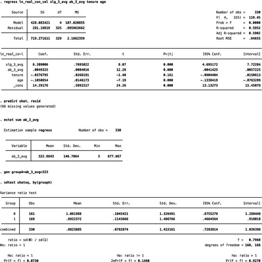
Assume for a moment that you’re estimating a model with the natural log of Major League Baseball players’ contract value as the dependent variable and several player characteristics as independent variables.
Three-year averages for slugging percentages (slg_3_avg) and at-bats (ab_3_avg), age, and tenure (the number of years a player has been with his current team) are the independent variables. You can arbitrarily divide the sample by the average number of at-bats. Players in Group A have below-average at-bats, and players in Group B have above-average at-bats.
The F-statistic in the figure, which shows the process of performing a GQ test in STATA, suggests that the difference in the RSS for the two groups is marginally significant in a one-tailed test (p-value = 0.0730).
A weakness of the GQ test is that the result is dependent on the criteria chosen for separating the sample measurements into their respective groups. This process is often quite arbitrary, so failing to find evidence of heteroskedasticity in one test doesn’t rule it out with different criteria used for separating the sample.
Consequently, the GQ test doesn’t provide any guidance for correcting or adjusting the model for heteroskedasticity, which is one reason why applied econometricians typically don’t rely on it in order to test for heteroskedasticity.
