


The cumulative density function (CDF) of a random variable X is the sum or accrual of probabilities up to some value. It shows how the sum of the probabilities approaches 1, which sometimes occurs at a constant rate and sometimes occurs at a changing rate.
The CDF for discrete random variables
For a discrete random variable, the CDF is equivalent to
where f(X) is the probability density function.
If you’re observing a discrete random variable, the CDF can be described in a table or graph. To construct a table, put the possible values of your random variable in one column, the probability that they will occur in another column, and the sums of the probabilities up to any given value in a third column.
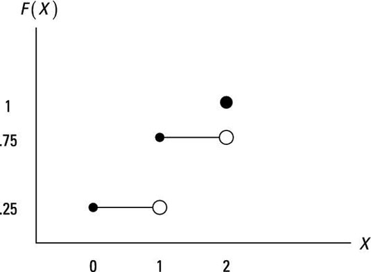
In a graphical depiction of the CDF, you place the possible values of the random variable on the horizontal axis, and the height of a horizontal line at each value shows the probability of that value summed with the probabilities of all smaller values.
Suppose you perform an experiment that consists of tossing two coins at the same time. You're interested in the number of times the coin lands heads up, so you designate the number of heads observed as my random variable X. The table illustrates the possible outcomes for this experiment and the values for X generated from the process.
| Outcome | First Coin | Second Coin | Number of Heads, X |
|---|---|---|---|
| 1 | T | T | 0 |
| 2 | T | H | 1 |
| 3 | H | T | 1 |
| 4 | H | H | 2 |
You can summarize the information with a table or graph of the CDF for X. The following table shows a tabular form of the CDF. Recall that the PDF, f(X), represents the probability of a given random event, and the CDF, F(X), is the sum of the probabilities up to any random value.
For example, f(X = 1) = 2/4 = 0.50 and F(X = 1) = 1/4 + 1/2 = 3/4 = 0.75.
| X | f(X) | F(X) |
|---|---|---|
| 0 | 0.25 | 0.25 |
| 1 | 0.50 | 0.75 |
| 2 | 0.25 | 1 |
The CDF for continuous random variables
Get ready for some calculus! The CDF is a sum of probabilities, and for a continuous function, finding a sum means integration. Integration is a calculus procedure that allows you to find densities under nonlinear functions. For a continuous random variable, the CDF is
where f(X) is the probability density function.
If you’re observing a continuous random variable, the CDF can be described in a function or graph. The function shows how the random variable behaves over any possible range of values.
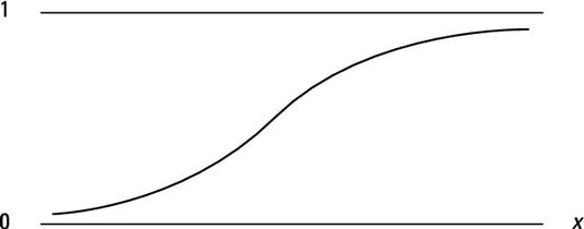
The precise shape of the CDF depends on the mean and variance (the square of the standard deviation) of your random variable. A smaller mean shifts the curve to the left, and a larger mean shifts the curve to the right. A smaller variance makes the curve steeper, whereas a larger variance makes the curve flatter.
