


Slicers are a new feature in Excel 2010 that you can use to filter your pivot tables. Slicers make it a snap to filter the contents of your pivot table on more than one field. Because slicers are Excel graphic objects (albeit some pretty fancy ones), you can move, resize, and delete them just as you would any other Excel graphic.
Click any cell in the pivot table.
Excel adds the PivotTable Tools contextual tab with the Options and Design tabs to the Ribbon.
On the PivotTable Tools Options tab, click the top of the Insert Slicer button in the Sort & Filter group.
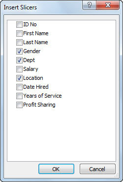
Excel opens the Insert Slicers dialog box with a list of all the fields in the active pivot table.
Select the check boxes for all the fields that you want to use in filtering the pivot table.
Excel will create a separate slicer for each of the selected fields.
Click OK.
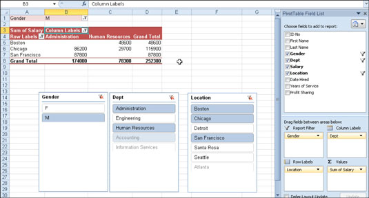
Excel displays slicers (as graphic objects) for each pivot table field you select. This figure shows a sample pivot table after using slicers created for the Gender, Dept, and Location fields to filter data so that only salaries for the men in the Administration and Human Resources departments in the Boston, Chicago, and San Francisco offices display.


