


Dynamic labels in Excel are labels that change according to the data you're viewing. With dynamic labeling, you can interactively change the labeling of data, consolidate many pieces of information into one location, and easily add layers of analysis.
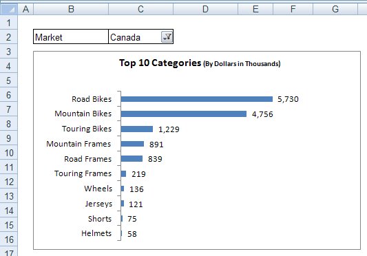
A common use for dynamic labels is labeling interactive charts. In the figure below, you see a pivot chart that shows the Top 10 Categories by market. When the market is changed in the Filter drop-down list, the chart changes. Now, wouldn't it be nifty to have a label on the chart itself that shows the market for which the data is currently being displayed?
To create a dynamic label within your chart, follow these steps:
On the Insert tab in the Ribbon, select the Text Box icon.
Click inside the chart to create an empty text box.
While the text box is selected, go up to the formula bar, type the equal sign (=), and then click the cell that contains the text for your dynamic label.
The text box is linked to cell C2. You'll notice that cell C2 holds the Filter drop-down list for the pivot table.

Format the text box so that it looks like any other label. You can format the text box using the standard formatting options found on the Home tab.
If all goes well, you'll have a label on your chart that changes to correspond with the cell to which it's linked. In the figure seen here, the France label within the chart is actually a dynamic label that changes when a new market is selected in the drop-down list.

What would happen if you were to link your text boxes to cells that contained formulas instead of simple labels? A whole new set of opportunities would open up. With text boxes linked to formulas, you could add a layer of analysis into your charts and dashboards without a lot of complex hocus pocus.
Take this simple example. Here, you see two views of the same pivot chart. On the top, the Northwest market is selected and you see that the pivot chart is labeled with a layer of analysis around Q4 variance. On the bottom, Southeast is selected and you can see that the label changes to correspond with the analysis around Q4 variance for the Southeast market.
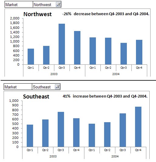
This example actually uses three dynamic labels. One to display the current selected market, one to display the actual calculation of Q4-2003 vs Q4-2003, and one to add some contextual text that describes the analysis.
Take a moment to examine what's happening here. The label showing 41% is linked to cell B13 which contains a formula returning the variance analysis. The label showing the contextual text is linked to cell C13, which contains an IF formula that returns a different sentence depending on whether the variance percent is an increase or decrease.
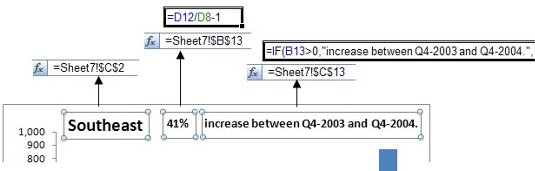
Together, these labels provide your audience with a clear message about the variance for the selected market. This is one of countless ways you can implement this technique.


