


The PV (Present Value), NPV (Net Present Value), and FV (Future Value) functions in Excel 2016 all found on the Financial button's drop-down menu on the Ribbon's Formulas tab (Alt+MI) enable you to determine the profitability of an investment.
Calculating the Present Value
The PV, or Present Value, function returns the present value of an investment, which is the total amount that a series of future payments is worth presently. The syntax of the PV function is as follows:
=PV(rate,nper,pmt,[fv],[type])
The fv and type arguments are optional arguments in the function (indicated by the square brackets). The fv argument is the future value or cash balance that you want to have after making your last payment. If you omit the fv argument, Excel assumes a future value of zero (0). The type argument indicates whether the payment is made at the beginning or end of the period: Enter 0 (or omit the type argument) when the payment is made at the end of the period, and use 1 when it is made at the beginning of the period.
The following figure contains several examples using the PV function. All three PV functions use the same annual percentage rate of 1.25 percent and term of 10 years. Because payments are made monthly, each function converts these annual figures into monthly ones. For example, in the PV function in cell E3, the annual interest rate in cell A3 is converted into a monthly rate by dividing by 12 (A3/12). The annual term in cell B3 is converted into equivalent monthly periods by multiplying by 12 (B3 x 12).
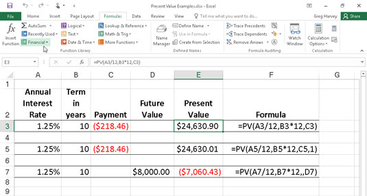
Note that although the PV functions in cells E3 and E5 use the rate, nper, and pmt ($218.46) arguments, their results are slightly different. This is caused by the difference in the type argument in the two functions: the PV function in cell E3 assumes that each payment is made at the end of the period (the type argument is 0 whenever it is omitted), whereas the PV function in cell E5 assumes that each payment is made at the beginning of the period (indicated by a type argument of 1). When the payment is made at the beginning of the period, the present value of this investment is $0.89 higher than when the payment is made at the end of the period, reflecting the interest accrued during the last period.
The third example in cell E7 (shown in Figure 4-1) uses the PV function with an fv argument instead of the pmt argument. In this example, the PV function states that you would have to make monthly payments of $7,060.43 for a 10-year period to realize a cash balance of $8,000, assuming that the investment returned a constant annual interest rate of 1 1/4 percent. Note that when you use the PV function with the fv argument instead of the pmt argument, you must still indicate the position of the pmt argument in the function with a comma (thus the two commas in a row in the function) so that Excel doesn't mistake your fv argument for the pmt argument.
Calculating the Net Present Value
The NPV function calculates the net present value based on a series of cash flows. The syntax of this function is
=NPV(<i>rate</i>,<i>value1</i>,[<i>value2</i>],[...])
where value1, value2, and so on are between 1 and 13 value arguments representing a series of payments (negative values) and income (positive values), each of which is equally spaced in time and occurs at the end of the period. The NPV investment begins one period before the period of the value1 cash flow and ends with the last cash flow in the argument list. If your first cash flow occurs at the beginning of the period, you must add it to the result of the NPV function rather than include it as one of the arguments.
The following figure illustrates the use of the NPV function to evaluate the attractiveness of a five-year investment that requires an initial investment of $30,000 (the value in cell G3). The first year, you expect a loss of $22,000 (cell B3); the second year, a profit of $15,000 (cell C3); the third year, a profit of $25,000 (cell D3); the fourth year, a profit of $32,000 (cell E3); and the fifth year, a profit of $38,000 (cell F3). Note that these cell references are used as the value arguments of the NPV function.
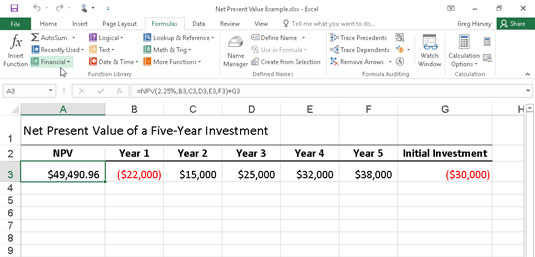
Unlike when using the PV function, the NPV function doesn't require an even stream of cash flows. The rate argument in the function is set at 2.25 percent. In this example, this represents the discount rate of the investment — that is, the interest rate that you may expect to get during the five-year period if you put your money into some other type of investment, such as a high-yield money-market account. This NPV function in cell A3 returns a net present value of $49,490.96, indicating that you can expect to realize a great deal more from investing your $30,000 in this investment than you possibly could from investing the money in a money-market account at the interest rate of 2.25 percent.
Calculating the Future Value
The FV function calculates the future value of an investment. The syntax of this function is
=FV(rate,nper,pmt,[pv],[type])
The rate, nper, pmt, and type arguments are the same as those used by the PV function. The pv argument is the present value or lump-sum amount for which you want to calculate the future value. As with the fv and type arguments in the PV function, both the pv and type arguments are optional in the FV function. If you omit these arguments, Excel assumes their values to be zero (0) in the function.
You can use the FV function to calculate the future value of an investment, such as an IRA (Individual Retirement Account). For example, suppose that you establish an IRA at age 43 and will retire 22 years from now at age 65 and that you plan to make annual payments into the IRA at the beginning of each year. If you assume a rate of return of 2.5 percent a year, you would enter the following FV function in your worksheet:
=FV(2.5%,22,–1500,,1)
Excel then indicates that you can expect a future value of $44,376.64 for your IRA when you retire at age 65. If you had established the IRA a year prior and the account already has a present value of $1,538, you would amend the FV function as follows:
=FV(2.5%,22,–1500,–1538,1)
In this case, Excel indicates that you can expect a future value of $47,024.42 for your IRA at retirement.


