


Excel Form controls are starting to look a bit dated, especially when paired with the modern-looking charts that come with Excel 2016. One clever way to alleviate this problem is to hijack the Slicer feature for use as a proxy Form control of sorts.
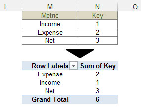
Create a simple table that holds the names you want for your controls, along with some index numbering.
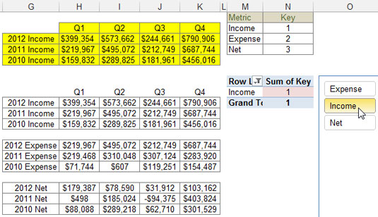
In this case, the table should contain three rows under a field called Metric. Each row should contain a metric name and an index number for each metric (Income, Expense, and Net).
Create a pivot table using that simple table.
Create a simple table that holds the names you want for your controls, along with some index numbering. After you have that, create a pivot table from it.
Place the cursor anywhere inside your newly created pivot table, click the Analyze tab, and then click the Insert Slicer icon.
The Insert Slicers dialog box appears.
Create a slicer for the Metric field.
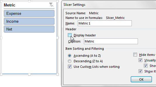
At this point, you have a slicer with the three metric names.
Right-click the slicer and choose Slicer Settings from the menu that appears.
The Slicer Settings dialog box appears.
Deselect the Display Header check box.
Each time you click the Metric slicer, the associated pivot table is filtered to show only the selected metric.
Creating a slicer for the Metric field and removing the header also filters the index number for that metric..
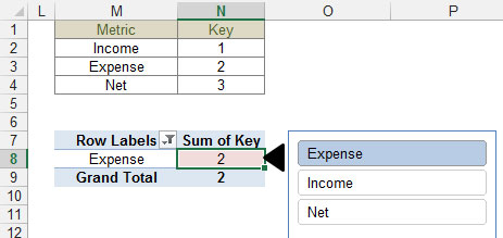
The filtered index number will always show up in the same cell (N8, in this case). So this cell can now be used as a trigger cell for VLOOKUP formulas, index formulas, IF statements, and so on.
Use the slicer-fed trigger cell (N8) to drive the formulas in your staging area.
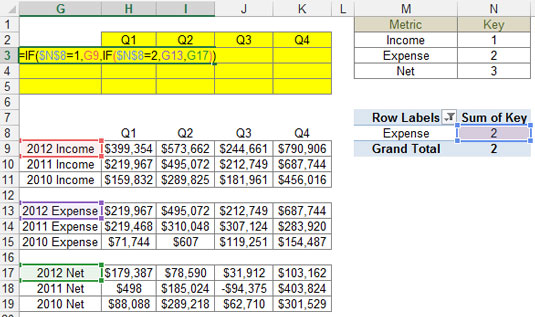
This formula tells Excel to check the value of cell N8. If the value of cell N8 is 1, which represents the value of the Income option, the formula returns the value in the Income dataset (cell G9). If the value of cell N8 is 2, which represents the value of the Expense option, the formula returns the value in the Expense dataset (cell G13). If the value of cell N8 is not 1 or 2, the value in cell G17 is returned.
Copy the formula down and across to build out the full staging table.
The final staging table is fed via the slicer.
The final step is to simply create a chart using the staging table as the source.
With this simple technique, you can provide your customers with an attractive interactive menu that more effectively adheres to the look and feel of their dashboards.


