


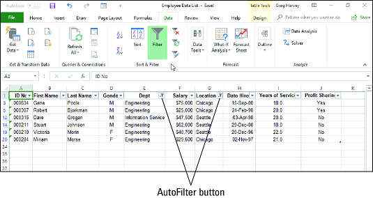
If you open a worksheet with a data list and you don’t find Excel’s AutoFilter buttons attached to each of the field names at the top of the list, you can display them simply by positioning the cell pointer in one of the cells with the field names and then clicking the Filter command button on the Ribbon’s Data tab or pressing Ctrl+Shift+L or Alt+AT.
The filter options on a column’s AutoFilter drop-down menu depend on the type of entries in the field. On the drop-down menu in a column that contains only date entries, the menu contains a Date Filters option to which a submenu of the actual filters is attached. On the drop-down menu in a column that contains only numeric entries (besides dates) or a mixture of dates with other types of numeric entries, the menu contains a Number Filters option. On the drop-down menu in a column that contains only text entries or a mixture of text, date, and other numeric entries, the menu contains a Text Filters option.Doing basic filtering in Excel 2019 by selecting specific field entries
In addition to the Date Filters, Text Filters, or Number Filters options (depending on the type of field), the AutoFilter drop-down menu for each field in the data list contains a list box with a complete listing of all entries made in that column, each with its own check box. At the most basic level, you can filter the data list by clearing the check box for all the entries whose records you don’t want to see in the list.This kind of basic filtering works best in fields such as City, State, or Country, which contain many duplicates, so you can see a subset of the data list that contains only the cities, states, or countries you want to work with at the time.
The easiest way to perform this basic type of filtering on a field is to first deselect the check box in front of the (Select All) option at the top of the field’s list box to clear the check boxes, and then select each of the check boxes containing the entries for the records you do want displayed in the filtered data list. After you finish selecting the check boxes for all the entries you want to keep, you click OK to close the AutoFilter drop-down menu.Excel then hides rows in the data list for all records except for those that contain the entries you just selected. The program also lets you know which field or fields have been used in the filtering operation by adding a cone filter icon to the column’s AutoFilter button. To restore all the records to the data list, you can remove the filtering by clicking the Clear command button in the Sort & Filter group of the Data tab of the Ribbon or by pressing Alt+AC.
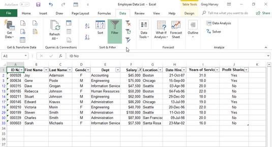
When doing this basic kind of list filtering, you can select specific entries from more than one field in this list. The following image illustrates this kind of situation. Here, I want only the employees in the company who work in the Engineering and Information Services departments in the Chicago and Seattle offices. To do this, I selected only the Engineering and Information Services entries in the list box on the Dept field’s AutoFilter drop-down menu and only the Chicago and Seattle entries in the list box on the Location field’s AutoFilter drop-down menu.
 The employee data list after filtering the Dept and Location fields.
As you can see above, after filtering the Employee data list so that only the records for employees in either the Engineering or Information Services department in either the Chicago or Seattle office locations are listed, Excel adds the cone filter icon to the AutoFilter buttons on both the Dept and Location fields in the top row, indicating that the list is filtered using criteria involving both fields.
Keep in mind that after filtering the data list in this manner, you can then copy remaining records that make up the desired subset of the data list to a new area in the same worksheet or to a new sheet in the workbook. You can then sort the data (by adding AutoFilter buttons with the Filter command button on the Data tab), chart the data, analyze the data, or summarize the data in an Excel pivot table.
Using the Text Filters options in Excel 2019
The AutoFilter drop-down menu for a field that contains only text or a combination of text, date, and numeric entries contains a Text Filters option that when you click or highlight displays its submenu containing the following options:- Equals: Opens the Custom AutoFilter dialog box with the Equals operator selected in the first condition.
- Does Not Equal: Opens the Custom AutoFilter dialog box with the Does Not Equal operator selected in the first condition.
- Begins With: Opens the Custom AutoFilter dialog box with the Begins With operator selected in the first condition.
- Ends With: Opens the Custom AutoFilter dialog box with the Ends With operator selected in the first condition.
- Contains: Opens the Custom AutoFilter dialog box with the Contains operator selected in the first condition.
- Does Not Contain: Opens the Custom AutoFilter dialog box with the Does Not Contain operator selected in the first condition.
- Custom Filter: Opens the Custom AutoFilter dialog box where you can select your own criteria for applying more complex AND or conditions.
Using the Date Filters options in Excel 2019
The AutoFilter drop-down menu for a field that contains only date entries contains a Date Filters option that when you click or highlight displays its submenu containing the following options:- Equals: Opens the Custom AutoFilter dialog box with the Equals operator selected in the first condition.
- Before: Opens the Custom AutoFilter dialog box with the Is Before operator selected in the first condition.
- After: Opens the Custom AutoFilter dialog box with the Is After operator selected in the first condition.
- Between: Opens the Custom AutoFilter dialog box with the Is After or Equal To operator selected in the first condition and the Is Before or Equal To operator selected in the second AND condition.
- Tomorrow: Filters the data list so that only records with tomorrow’s date in this field are displayed in the worksheet.
- Today: Filters the data list so that only records with the current date in this field are displayed in the worksheet.
- Yesterday: Filters the data list so that only records with yesterday’s date in this field are displayed in the worksheet.
- Next Week: Filters the data list so that only records with date entries in the week ahead in this field are displayed in the worksheet.
- This Week: Filters the data list so that only records with date entries in the current week in this field are displayed in the worksheet.
- Last Week: Filters the data list so that only records with date entries in the previous week in this field are displayed in the worksheet.
- Next Month: Filters the data list so that only records with date entries in the month ahead in this field are displayed in the worksheet.
- This Month: Filters the data list so that only records with date entries in the current month in this field are displayed in the worksheet.
- Last Month: Filters the data list so that only records with date entries in the previous month in this field are displayed in the worksheet.
- Next Quarter: Filters the data list so that only records with date entries in the three-month quarterly period ahead in this field are displayed in the worksheet.
- This Quarter: Filters the data list so that only records with date entries in the current three-month quarterly period in this field are displayed in the worksheet.
- Last Quarter: Filters the data list so that only records with date entries in the previous three-month quarterly period in this field are displayed in the worksheet.
- Next Year: Filters the data list so that only records with date entries in the calendar year ahead in this field are displayed in the worksheet.
- This Year: Filters the data list so that only records with date entries in the current calendar year in this field are displayed in the worksheet.
- Last Year: Filters the data list so that only records with date entries in the previous calendar year in this field are displayed in the worksheet.
- Year to Date: Filters the data list so that only records with date entries in the current year up to the current date in this field are displayed in the worksheet.
- All Dates in the Period: Filters the data list so that only records with date entries in the quarter (Quarter 1 through Quarter 4) or month (January through December) that you choose from its submenu are displayed in the worksheet.
- Custom Filter: Opens the Custom AutoFilter dialog box where you can select your own criteria for more complex AND or conditions.
When selecting dates for conditions using the Equals, Is Before, Is After, Is Before or Equal To, or Is After or Equal To operator in the Custom AutoFilter dialog box, you can select the date by clicking the Date Picker button (the one with the calendar icon) and then clicking the specific date on the drop-down date palette. When you open the date palette, it shows the current month and the current date selected. To select a date in an earlier month, click the Previous button (the one with the triangle pointing left) until its month is displayed in the palette. To select a date in a later month, click the Next button (the one with the triangle pointing right) until its month is displayed in the palette.
Using the Number Filters options in Excel 2019
The AutoFilter drop-down menu for a field that contains only number entries besides dates or a combination of dates and other numeric entries contains a Number Filters option that when you click or highlight it displays its submenu containing the following options:- Equals: Opens the Custom AutoFilter dialog box with the Equals operator selected in the first condition.
- Does Not Equal: Opens the Custom AutoFilter dialog box with the Does Not Equal operator selected in the first condition.
- Greater Than: Opens the Custom AutoFilter dialog box with the Is Greater Than operator selected in the first condition.
- Greater Than or Equal To: Opens the Custom AutoFilter dialog box with the Is Greater Than or Equal To operator selected in the first condition.
- Less Than: Opens the Custom AutoFilter dialog box with the Is Less Than operator selected in the first condition.
- Less Than or Equal To: Opens the Custom AutoFilter dialog box with the Is Less Than or Equal to operator selected in the first condition.
- Between: Opens the Custom AutoFilter dialog box with the Is Greater Than or Equal To operator selected in the first condition and the Is Less Than or Equal To operator selected in the second AND condition.
- Top 10: Opens the Top 10 AutoFilter dialog box so that you can filter the list to just the ten or so top or bottom values or percentages in the field.
- Above Average: Filters the data list to display only records where the values in the field are greater than the average of the values in this field.
- Below Average: Filters the data list to display only records where the values in the field are less than the average of the values in this field.
- Custom Filter: Opens the Custom AutoFilter dialog box where you can select your own criteria for more complex AND or conditions.
Making it to the Top Ten!
The Top Ten option on the Number Filters option’s submenu enables you to filter out all records except those whose entries in that field are at the top or bottom of the list by a certain number (10 by default) or in a certain top or bottom percent (10 by default). Of course, you can only use the Top Ten item in numerical fields and date fields; this kind of filtering doesn’t make any sense when you’re dealing with entries in a text field.When you click the Top Ten option on the Number Filters option’s submenu, Excel opens the Top 10 AutoFilter dialog box where you can specify your filtering criteria. By default, the Top 10 AutoFilter dialog box is set to filter out all records except those whose entries are among the top ten items in the field by selecting Top in the drop-down list box on the left, 10 in the middle combo box, and Items in the drop-down list box on the right. If you want to use these default criteria, you simply click OK in the Top 10 AutoFilter dialog box.
The image below shows you the sample employee data list after using the Top 10 Items AutoFilter to display only the records with the top ten salaries in the data list.
 Using the Top 10 Items AutoFilter to filter out all records except for those with the top ten salaries.
You can also change the filtering criteria in the Top 10 AutoFilter dialog box before you filter the data. You can choose between Top and Bottom in the leftmost drop-down list box and between Items and Percent in the rightmost one. You can also change the number in the middle combo box by clicking it and entering a new value or using the spinner buttons to select one.
Filtering an Excel data list on a field’s font and fill colors or cell icons
Just as you can sort a data list using the font or fill color or cell icons that you’ve assigned with the Conditional Formatting feature to values in the field that are within or outside of certain parameters, you can also filter the list.To filter a data list on a font color, fill color, or cell icon used in a field, you click its AutoFilter button and then select the Filter by Color option from the drop-down menu. Excel then displays a submenu from which you choose the font color, fill color, or cell icon to use in the sort:
- To filter the data list so that only the records with a particular font color in the selected field — assigned with the Conditional Formatting Highlight Cell Rules or Top/Bottom Rules options — appear in the list, click its color swatch in the Filter by Font Color submenu.
- To filter the data list so that only the records with a particular fill color in the selected field — assigned with the Conditional Formatting Highlight Cell Rules, Top/Bottom Rules, Data Bars, or Color Scales options — appear in the list, click its color swatch in the Filter by Font Color submenu.
- To filter the data list so that only the records with a particular cell icon in the selected field — assigned with the Conditional Formatting Icon Sets options — appear in the list, click the icon in the Filter by Cell Icon submenu.


