


In the course of creating and editing a worksheet in Excel 2013, you may find that you need to modify the worksheet display many times as you work with the document. Excel’s Custom Views feature enables you to save any of these types of changes to the worksheet display.
This way, instead of taking the time to manually set up the worksheet display that you want, you can have Excel re-create it for you simply by selecting the view.
When you create a view, Excel can save any of the following settings: the current cell selection, print settings (including different page setups), column widths and row heights (including hidden columns), display settings on the Advanced tab of the Excel Options dialog box, as well as the current position and size of the document window and the window pane arrangement (including frozen panes).
To create a custom view of your worksheet, follow these steps:
Make all the necessary changes to the worksheet display so that the worksheet window appears exactly as you want it to appear each time you select the view.
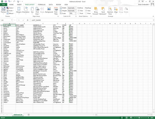
Also select all the print settings on the Page Layout tab that you want used in printing the view.
Click the Custom Views command button in the Workbook Views group at the beginning of the View tab or press Alt+WC.
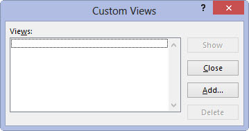
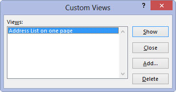
This action opens the Custom Views dialog box, where you add the view that you’ve just set up in the worksheet.
Click the Add button.
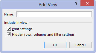
This action opens the Add View dialog box, where you type a name for your new view.
Enter a unique descriptive name for your view in the Name text box.
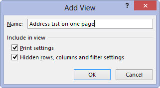
Make sure that the name you give the view reflects all its pertinent settings.
To include print settings and hidden columns and rows in your view, leave the Print Settings and Hidden Rows, Columns and Filter Settings check boxes selected when you click the OK button.
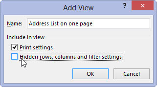
If you don’t want to include these settings, clear the check mark from either one or both of these check boxes before you click OK.
When you click OK, Excel closes the Custom Views dialog box. When you next open this dialog box, the name of your new view appears in the Views list box.
Click the Close button to close the Custom Views dialog box.
Custom views are saved as part of the workbook file. To be able to use them whenever you open the spreadsheet for editing, you need to save the workbook with the new view.
Click the Save button on the Quick Access toolbar or press Ctrl+S to save the new view as part of the workbook file.
After you create your views, you can display the worksheet in that view at any time while working with the spreadsheet.


