


Use the AutoFilter feature in Excel 2010 to hide everything in a table except the records you want to view. Filtering displays a subset of a table, providing you with an easy way to break down your data into smaller, more manageable chunks. Filtering does not rearrange your data; it simply temporarily hides rows that don't match the criteria you specify.
Click inside a table, and then choose Filter in the Sort & Filter group of the Data tab (or press Ctrl+Shift+L).
Filter arrows appear beside the column headings. If the data is formatted as an Excel table, skip this step; you should already see the filter arrows.
Click the filter arrow beside the column heading for the column you want to filter.
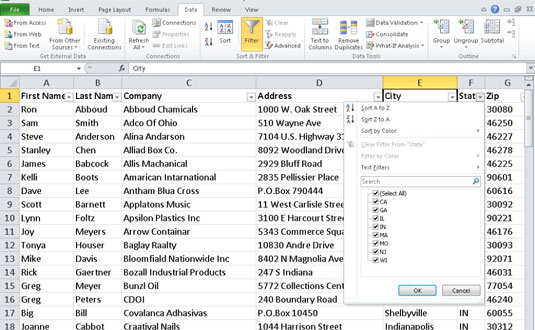
Excel displays a drop-down list, which includes one of each unique entry from the selected column.
Remove the check mark from Select All.
All items in the list are deselected.
Select the check box for the entry you want to filter and then click OK.
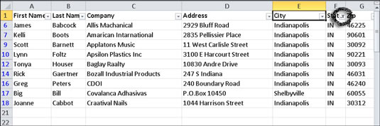
You can select multiple check boxes to filter on two or more items. Excel displays only the records that match your selections.
(Optional) Repeat Steps 2–4 as needed to apply additional filters to other columns in the filtered data.
You can apply filters to multiple columns in a table to further isolate specific items. Notice that the filter arrows on filtered columns take on a different appearance to indicate that a filter is in use.


