


To create a two-variable data table to perform what-if analysis in Excel 2010, you enter two ranges of possible input values for the same formula: a range of values for the Row Input Cell in the Data Table dialog box across the first row of the table and a range of values for the Column Input Cell in the dialog box down the first column of the table. You then enter the formula (or a copy of it) in the cell located at the intersection of this row and column of input values.
The steps below for creating a two-variable data table follow a specific example (rather than using generic steps) to help you understand exactly how to use this feature. The following figure shows a Sales Projections worksheet in which two variables are used in calculating the projected sales for the year 2011: a growth rate as a percentage of increase over last year's sales (in cell B3) and expenses calculated as a percentage of last year's sales (in cell B4). The formula in cell B5 is: =B2+(B2*B3)-(B2*B4).
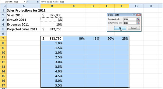
The column of possible growth rates ranging from 1% to 5.5% is entered down column B in the range B8:B17, and a row of possible expenses percentages is entered in the range C7:F7. Follow these steps to complete the two-variable data table for this example:
Copy the original formula entered in cell B5 into cell B7 by typing = (equal to) and then clicking cell B5.
For a two-variable data table, the copy of the original formula must be entered at the intersection of the row and column input values.
Select the cell range B7:F17.
The range of the data table includes the formula along with the various growth rates.
Choose What-If Analysis→Data Table in the Data Tools group on the Data tab.
Excel opens the Data Table dialog box with the insertion point in the Row Input Cell text box.
Click cell B4 to enter the absolute cell address, $B$4, in the Row Input Cell text box.
Click the Column Input Cell text box and then click cell B3 to enter the absolute cell address, $B$3, in this text box.
Click OK.
Excel fills the blank cells of the data table with a TABLE formula using B4 as the Row Input Cell and B3 as the Column Input Cell.
 Sales projection worksheet after creating the two-variable data table in the range C8:F17.
The array formula {=TABLE(B4,B3)} that Excel creates for the two-variable data table in this example specifies both a Row Input Cell argument (B4) and a Column Input Cell argument (B3). Because this single array formula is entered into the entire data table range of C8:F17, keep in mind that any editing (in terms of moving or deleting) is restricted to the entire range.


