Analyze an RLC Second-Order Parallel Circuit Using Duality

Second-order RLC circuits have a resistor, inductor, and capacitor connected serially or in parallel. To analyze a second-order parallel circuit, you follow the same process for analyzing an RLC series circuit.

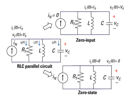
Here is an example RLC parallel circuit. The left diagram shows an input i_N with initial inductor current I₀ and capacitor voltage V₀. The top-right diagram shows the input current source i_N set equal to zero, which lets you solve for the zero-input response. The bottom-right diagram shows the initial conditions (I₀ and V₀) set equal to zero, which lets you obtain the zero-state response.

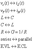
With duality, you substitute every electrical term in an equation with its dual, or counterpart, and get another correct equation. For example, voltage and current are dual variables.

Set up a typical RLC parallel circuit

Because the components of the sample parallel circuit shown earlier are connected in parallel, you set up the second-order differential equation by using Kirchhoff’s current law (KCL). KCL says the sum of the incoming currents equals the sum of the outgoing currents at a node. Using KCL at Node A of the sample circuit gives you

i_N(t) =i_R(t) +i_C(t) +i_L(t)

Next, put the resistor current and capacitor current in terms of the inductor current. The resistor current i_R(t) is based on the old, reliable Ohm’s law:

The element constraint for an inductor is given as

The current i_L(t) is the inductor current, and L is the inductance. This constraint means a changing current generates an inductor voltage. If the inductor current doesn’t change, there’s no inductor voltage, implying a short circuit.

Parallel devices have the same voltage v(t). You use the inductor voltage v(t) that’s equal to the capacitor voltage to get the capacitor current i_C(t):

Now substitute v(t) = Ldi_L(t)/dt into Ohm’s law, because you also have the same voltage across the resistor and inductor:

Substitute the values of i_R(t) and i_C(t) into the KCL equation to give you the device currents in terms of the inductor current:

The RLC parallel circuit is described by a second-order differential equation, so the circuit is a second-order circuit. The unknown is the inductor current i_L(t).

The analysis of the RLC parallel circuit follows along the same lines as the RLC series circuit. Compare the preceding equation with this second-order equation derived from the RLC series:

The two differential equations have the same form. The unknown solution for the parallel RLC circuit is the inductor current, and the unknown for the series RLC circuit is the capacitor voltage. These unknowns are dual variables.

With duality, you can replace every electrical term in an equation with its dual and get another correct equation. If you use the following substitution of variables in the differential equation for the RLC series circuit, you get the differential equation for the RLC parallel circuit.

Duality allows you to simplify your analysis when you know prior results. Yippee!

Find the zero-input response

The results you obtain for an RLC parallel circuit are similar to the ones you get for the RLC series circuit. For a parallel circuit, you have a second-order and homogeneous differential equation given in terms of the inductor current:

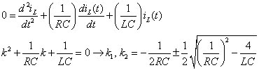
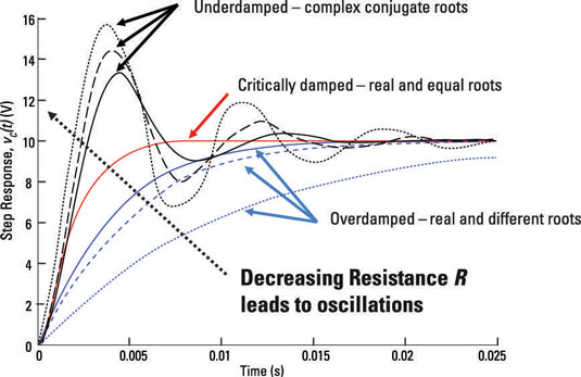
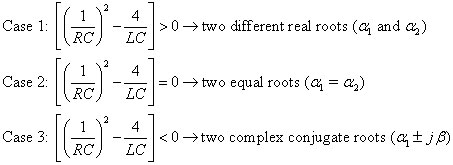
The preceding equation gives you three possible cases under the radical:

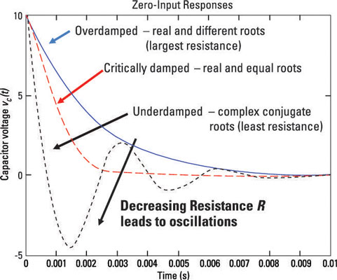
The zero-input responses of the inductor responses resemble the form shown here, which describes the capacitor voltage.

When you have k₁ and k₂, you have the zero-input response i_ZI(t). The solution gives you

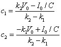
You can find the constants c₁ and c₂ by using the results found in the RLC series circuit, which are given as

Apply duality to the preceding equation by replacing the voltage, current, and inductance with their duals (current, voltage, and capacitance) to get c₁ and c₂ for the RLC parallel circuit:

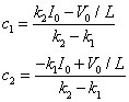
After you plug in the dual variables, finding the constants c₁ and c₂ is easy.

Arrive at the zero-state response

Zero-state response means zero initial conditions. You need to find the homogeneous and particular solutions of the inductor current when there’s an input source i_N(t). Zero initial conditions means looking at the circuit when there’s 0 inductor current and 0 capacitor voltage.

When t < 0, u(t) = 0. The second-order differential equation becomes the following, where i_L(t) is the inductor current:

For a step input where u(t) = 0 before time t = 0, the homogeneous solution ih(t) is

Adding the homogeneous solution to the particular solution for a step input IAu(t) gives you the zero-state response i_ZS(t):

Now plug in the values of i_h(t) and i_p(t):

Here are the results of C₁ and C₂ for the RLC series circuit:

You now apply duality through a simple substitution of terms in order to get C₁ and C₂ for the RLC parallel circuit:

Find the total response

You finally add up the zero-input response i_ZI(t) and the zero-state response i_ZS(t) to get the total response i_L(t):

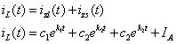
The solution resembles the results for the RLC series circuit. Also, the step responses of the inductor current follow the same form as the ones shown in the step responses found in this sample circuit, for the capacitor voltage.