


Interested in a new Raspberry Pi project? The Lorenz attractor almost singlehandedly originated a whole branch of science chaos theory. It seems fitting that a man who worked for so much of his life in Cambridge, Massachusetts, be remembered for a program that runs on an operating system designed in Cambridge, England.
Edward Norton Lorenz was working on systems to predict the weather. He had constructed a simple mathematical model of how the atmosphere convection should behave. It boiled down to a system of three ordinary differential equations. He was using one of the earliest computers in the 1950s to solve these equations by numerical methods because there is no analytical way to solve them. This involved repeated calculations or iterations of values in order to home in on the result. The output of one set of calculations was fed into the input of another. This is a well-known technique first invented by Isaac Newton; the results either home in on the correct answer, getting smaller and smaller, or shoot off into infinity.
What Lorenz found was a class of equations that neither homed in on one result nor shot off to infinity but did something in between. It produced what appeared to be a cycling result with the same values repeating in a pattern. However, closer inspection revealed that although the results did cycle, they never repeated — in other words, they cycled without end but stayed within certain bounds. A sort of never-ending, never-repeating finite set of numbers.
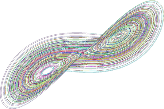
This pattern of numbers consisted of three values that would change with respect to each other. If you were to use these numbers to plot a position in three-dimensional space, they would describe a line or orbit that never repeated but went on forever. This shape was later christened a fractal, and this class of fractals is known as a strange attractor. No matter what the initial starting conditions were, the equations always ended up on this curve (hence, the name attractor, and because it’s an odd thing to happen, the word strange).
The shape of this curve is a twisted figure-eight loop known as a butterfly curve or the Lorenz attractor. In 1969, Lorenz described the butterfly effect, which states that an almost insignificant change in initial conditions (like the beating of a butterfly’s wings) could cause a large change in the outcome of an iterated system.
All that Lorenz had to visualize his numbers with was a crude teleprinter, but these days we have high-speed computers with graphic displays Lorenz never dreamed of. It’s comparatively easy to see his curve in more detail than Lorenz ever could.
The implementation of the BASIC language in RISC OS makes it easy to write a program to display the Lorenz attractor very quickly and in great detail. This is shown in the following code.
   10 : REM The Lorenz Attractor - by Mike Cook
   20 : MODE 28
   30 : CLS:CLG
   40 : PROC_Size
   50 : S=Ymax%/80:SX=Xmax%/70:SZ=2
   60 : N%=70:F%=0:INC=4E-3
   70 : SX%=Xmax%/2:SY%=Ymax%/2:SZ%=0
   80 : X=-6.5:Y=-8.8:Z=20
   90 : P1=10:P2=28:P3=2.66666
   100 :
   110 : REPEAT
   120 : N%=N%+1
   130 : IF N%>200 THEN N%=0:GCOL 0,RND(63) TINT 255
   140 : D1=P1*(Y-X)
   150 : D2=P2*X-Y-X*Z
   160 : D3=X*Y-P3*Z
   170 : X=X+D1*INC
   180 : Y=Y+D2*INC
   190 : Z=Z+D3*INC
   200 : PROC_PLOT(X,Y)
   210 : TIME=0
   220 : REPEAT
   230 : UNTIL TIME>0
   240 : B%=ADVAL(-1)
   250 : UNTIL B%<>0
   260 : A$=GET$
   270 : IF A$ ="s" THEN *ScreenSave Attract
   280 : END
   290 :
   300 : DEF PROC_PLOT(X,Y)
   310 : X%=X*SX:Y%=Y*S
   320 : X%=X%+SX%:Y%=Y%+SY%
   330 : IF F% = 0 THEN MOVE X%,Y% ELSE DRAW X%,Y%
   340 : F%=1 : REM move only the first time
   350 : ENDPROC
   360 :
   370 : DEF PROC_Size
   380 : SYS"OS_ReadModeVariable",-1,3 TO ,,Ncolours%
   390 : SYS"OS_ReadModeVariable",-1,4 TO ,,Xfact%
   400 : SYS"OS_ReadModeVariable",-1,5 TO ,,Yfact%
   410 : SYS"OS_ReadModeVariable",-1,11 TO ,,XLim%
   420 : SYS"OS_ReadModeVariable",-1,12 TO ,,YLim%
   430 : Xmax%=XLim%<<Xfact%
   440 : Ymax%=YLim%<<Yfact%
   450 : VDU 5
   460 : ENDPROC
The initial starting positions are given in line 80, and the parameters of the equation are given in line 90. The main loop in the program goes from line 110 to line 280. This simply repeats until you press any keyboard key. If the key you press is an S, then a screen dump is done to save a picture of the screen in sprite format. The loop works by lines 140 to 160 finding the difference in values from the last to the present iteration. The iteration calculation is then scaled with the variable INC, which is set to be 0.004 in lines 170 to 190, and the resultant number is plotted on the screen. Notice how only the x and y values are plotted, giving a view looking into the z-axis. You can change the two variables passed in the PROC PLOT call to be any two values to get a different view on the curve. You can combine the x, y, and z values in this call to give any angle of orthographic projection if you like. For example, making the following changes to the code will give an isometric view of the curve:
   42  : C1= 0.707107 : C2 = 0.408241
   43  : C3 = 0.816597 : C4 = -C2
   200 : PROC_PLOT(C1*X + C1*Z, C2*X + C3*Y + C4*Z)
Lines 210 to 230 simply make a time delay, making it longer by increasing the number at the end of line 230 or eliminating it altogether by skipping these three lines.
The PLOT procedure itself simply scales the two points and then shifts them to the middle of the screen. Finally, if it’s the first time plotting, it gives a move command; otherwise, it gives a draw from the last point graphics command.
The Size procedure gets the size of the screen in pixels so the graph fills the screen, and lines 120 and 130 add a bit of variety by changing the line’s color every 200 points.


