
Creating an Excel chart on a separate chart sheet
Sometimes you know you want your new Excel chart to appear on its own separate sheet in the workbook and you don’t have time to fool around with moving an embedded chart created with the Quick Analysis tool or the various chart command buttons on the Insert tab of the Ribbon to its own sheet. In such a situation, simply position the cell pointer somewhere in the table of data to be graphed (or select the specific cell range in a larger table) and then just press F11.Excel then creates a clustered column chart using the table’s data or cell selection on its own chart sheet (Chart1) that precedes all the other sheets in the workbook below. You can then customize the chart on the new chart sheet as you would an embedded chart.
 Clustered column chart created on its own chart sheet.
Refining your Excel chart from the Design tab
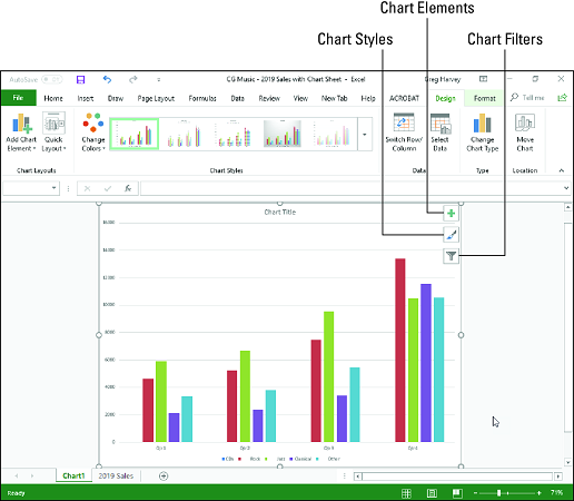
You can use the command buttons on the Design tab of the Chart Tools contextual tab to make all kinds of changes to your new Excel chart. This tab contains the following command buttons:- Chart Layouts: Click the Add Chart Element button to select the type of chart element you want to add. (You can also do this by selecting the Chart Elements button in the upper-right corner of the chart itself.) Click the Quick Layout button and then click the thumbnail of the new layout style you want applied to the selected chart on the drop-down gallery.
- Chart Styles: Click the Change Colors button to open a drop-down gallery and then select a new color scheme for the data series in the selected chart. In the Chart Styles gallery, highlight and then click the thumbnail of the new chart style you want applied to the selected chart. Note that you can select a new color and chart style in the opened galleries by clicking the Chart Styles button in the upper-right corner of the chart itself.
- Switch Row/Column: Click this button to immediately interchange the worksheet data used for the Legend Entries (series) with that used for the Axis Labels (Categories) in the selected chart.
- Select Data: Click this button to open the Select Data Source dialog box, where you can not only modify which data is used in the selected chart but also interchange the Legend Entries (series) with the Axis Labels (Categories), but also edit out or add particular entries to either category.
- Change Chart Type: Click this button to change the type of chart and then click the thumbnail of the new chart type on the All Charts tab in the Change Chart dialog box, which shows all kinds of charts in Excel.
- Move Chart: Click this button to open the Move Chart dialog box, where you move an embedded chart to its own chart or move a chart on its own sheet to one of the worksheets in the workbook as an embedded chart.
Modifying chart layout and style of your Excel chart
As soon as Excel draws a new chart in your worksheet, the program selects your chart and adds the Chart Tools contextual tab to the end of the Ribbon and selects its Design tab. You can then use the Quick Layout and Chart Styles galleries to further refine the new chart.The image below shows the original clustered column chart after selecting Layout 9 on the Quick Layout button’s drop-down gallery and then selecting the Style 8 thumbnail on the Chart Styles drop-down gallery. Selecting Layout 9 adds Axis Titles to both the vertical and horizontal axes as well as creating the Legend on the right side of the graph. Selecting Style 8 gives the clustered column chart its dark background and contoured edges on the clustered columns themselves.
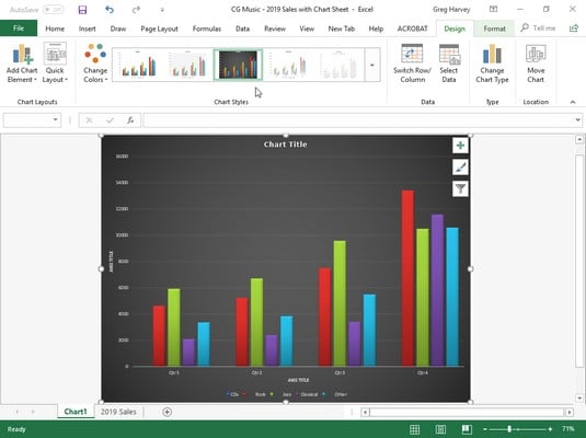 Clustered column chart on its own chart sheet after selecting a new layout and style from the Design tab.
Switching the rows and columns in an Excel chart
Normally when Excel creates a new chart, it automatically graphs the data by rows in the cell selection so that the column headings appear along the horizontal (category) axis at the bottom of the chart and the row headings appear in the legend (assuming that you’re dealing with a chart type that utilizes an x- and y-axis).You can click the Switch Row/Column command button on the Design tab of the Chart Tools contextual tab to switch the chart so that row headings appear on the horizontal (category) axis and the column headings appear in the legend (or you can press Alt+JCW).
You see how this works in the image below. The following image shows the same clustered column chart after selecting the Switch Row/Column command button on the Design tab. Now, column headings (Qtr 1, Qtr 2, Qtr 3, and Qtr 4) are used in the legend on the right and the row headings (Genre, Rock, Jazz, Classical, and Other) appear along the horizontal (category) axis.
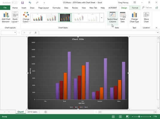 The clustered column chart after switching the columns and rows.
Editing the source of the data graphed in the Excel chart
When you click the Select Data command button on the Design tab of the Chart Tools contextual tab (or press Alt+JCE), Excel opens a Select Data Source dialog box similar to the one shown below. The controls in this dialog box enable you to make the following changes to the source data:- Modify the range of data being graphed in the chart by clicking the Chart Data Range text box and then making a new cell selection in the worksheet or typing in its range address.
- Switch the row and column headings back and forth by clicking its Switch Row/Column button.
- Edit the labels used to identify the data series in the legend or on the horizontal (category) by clicking the Edit button on the Legend Entries (Series) or Horizontal (Categories) Axis Labels side and then selecting the cell range with appropriate row or column headings in the worksheet.
- Add additional data series to the chart by clicking the Add button on the Legend Entries (Series) side and then selecting the cell containing the heading for that series in the Series Name text box and the cells containing the values to be graphed in that series in the Series Values text box.
- Delete a label from the legend by clicking its name in the Legend Entries (Series) list box and then clicking the Remove button.
- Modify the order of the data series in the chart by clicking the series name in the Legend Entries (Series) list box and then clicking the Move Up button (the one with the arrow pointing upward) or the Move Down button (the one with the arrow pointing downward) until the data series appears in the desired position in the chart.
- Indicate how to deal with empty cells in the data range being graphed by clicking the Hidden and Empty Cells button and then selecting the appropriate Show Empty Cells As option button (Gaps, the default; Zero and Connect Data Points with Line, for line charts). Click the Show Data in Hidden Rows and Columns check box to have Excel graph data in the hidden rows and columns within the selected chart data range.
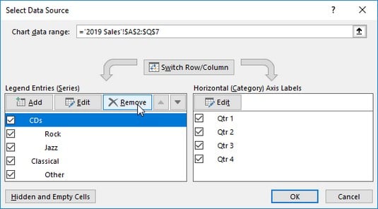 Using the Select Data Source dialog box to remove the empty Genre label from the legend of the clustered column chart.
The example clustered column chart in the two images provided above illustrates a common situation where you need to use the options in the Source Data Source dialog box. The worksheet data range for this chart, A2:Q7, includes the Genre row heading in cell A3 that is essentially a heading for an empty row (E3:Q3). As a result, Excel includes this empty row as the first data series in the clustered column chart. However, because this row has no values in it (the heading is intended only to identify the type of music download recorded in that column of the sales data table), its cluster has no data bars (columns) in it — a fact that becomes quite apparent when you switch the column and row headings.
To remove this empty data series from the clustered column chart, you follow these steps:
- Click the Chart1 sheet tab and then click somewhere in the chart area to select the clustered column chart; click the Design tab under Chart Tools on the Ribbon and then click the Select Data command button on the Design tab of the Chart Tools contextual tab.
Excel opens the Select Data Source dialog box in the 2016 Sales worksheet similar to the one shown above.
- Click the Switch Row/Column button in the Select Data Source dialog box to place the row headings (Genre, Rock, Jazz, Classical, and Other) in the Legend Entries (Series) list box.
- Click Genre at the top of the Legend Entries (Series) list box and then click the Remove button.
Excel removes the empty Genre data series from the clustered column chart as well as removing the Genre label from the Legend Entries (Series) list box in the Select Data Source dialog box.
- Click the Switch Row/Column button in the Select Data Source dialog box again to exchange the row and column headings in the chart and then click the Close button to close the Select Data Source dialog box.
After you close the Select Data Source dialog box, you will notice that the various colored outlines in the chart data range no longer include row 3 with the Genre row heading (A3) and its empty cells (E3:Q3).
Instead of going through all those steps in the Select Data Source dialog box to remove the empty Genre data series from the example clustered column chart, you can simply remove the Genre series from the chart on the Chart Filters button pop-up menu. When the chart’s selected, click the Chart Filters button in the upper-right corner of the chart (with the cone filter icon) and then deselect the Genre check box that appears under the SERIES heading on the pop-up menu before clicking the Apply button. As soon as you click the Chart Filters button to close its menu, you see that Excel has removed the empty data series from the redrawn clustered column chart. Read here to find out about Excel filters.