


 Some great data, but how do you make sense of it?
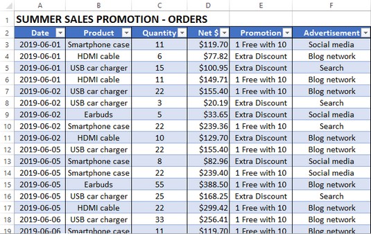
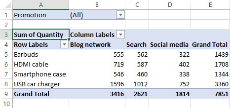
This table contains well over 100 records, each of which is an order from a sales promotion. That’s not a ton of data in the larger scheme of things, but trying to make sense of even this relatively small data set just by eyeballing the table’s contents is futile. For example, how many earbuds were sold via social media advertising? Who knows? Ah, but now look at the image below, which shows an Excel PivotTable built from the order data. This report tabulates the number of units sold for each product based on each promotion. From here, you can quickly see that 322 earbuds were sold via social media advertising. That is what PivotTables do.
 The PivotTable creates order out of data chaos.
PivotTables help you analyze large amounts of data by performing three operations: grouping the data into categories; summarizing the data using calculations; and filtering the data to show just the records you want to work with:
- Grouping: A PivotTable is a powerful data-analysis tool in part because it automatically groups large amounts of data into smaller, more manageable chunks. For example, suppose you have a data source with a Region field in which each item contains one of four values: East, West, North, and South. The original data may contain thousands of records, but if you build your PivotTable using the Region field, the resulting table has just four rows — one each for the four unique Region values in your data.
You can also create your own grouping after you build your PivotTable. For example, if your data has a Country field, you can build the PivotTable to group all the records that have the same Country value. When you have done that, you can further group the unique Country values into continents: North America, South America, Europe, and so on.
- Summarizing: In conjunction with grouping data according to the unique values in one or more fields, Excel also displays summary calculations for each group. The default calculation is Sum, which means that for each group, Excel totals all the values in some specified field. For example, if your data has a Region field and a Sales field, a PivotTable can group the unique Region values and display the total of the Sales values for each one. Excel has other summary calculations, including Count, Average, Maximum, Minimum, and Standard Deviation.
Even more powerful, a PivotTable can display summaries for one grouping broken down by another. For example, suppose your sales data also has a Product field. You can set up a PivotTable to show the total Sales for each Product, broken down by Region.
- Filtering: A PivotTable also enables you to view just a subset of the data. For example, by default, the PivotTable’s groupings show all the unique values in the field. However, you can manipulate each grouping to hide those that you do not want to view. Each PivotTable also comes with a report filter that enables you to apply a filter to the entire PivotTable. For example, suppose your sales data also includes a Customer field. By placing this field in the PivotTable’s report filter, you can filter the PivotTable report to show just the results for a single Customer.
Excel PivotTable features
You can get up to speed with PivotTables very quickly after you learn a few key concepts. You need to understand the features that make up a typical PivotTable, particularly the four areas — row, column, data, and filter — to which you add fields from your data. Check out the following PivotTable features:- Row area: Displays vertically the unique values from a field in your data.
- Column area: Displays horizontally the unique values from a field in your data.
- Value area: Displays the results of the calculation that Excel applied to a numeric field in your data.
- Row field header: Identifies the field contained in the row area. You also use the row field header to filter the field values that appear in the row area.
- Column field header: Identifies the field contained in the column area. You also use the column field header to filter the field values that appear in the column area.
- Value field header: Specifies both the calculation (such as Sum) and the field (such as Quantity) used in the value area.
- Filter area: Displays a drop-down list that contains the unique values from a field. When you select a value from the list, Excel filters the PivotTable results to include only the records that match the selected value.
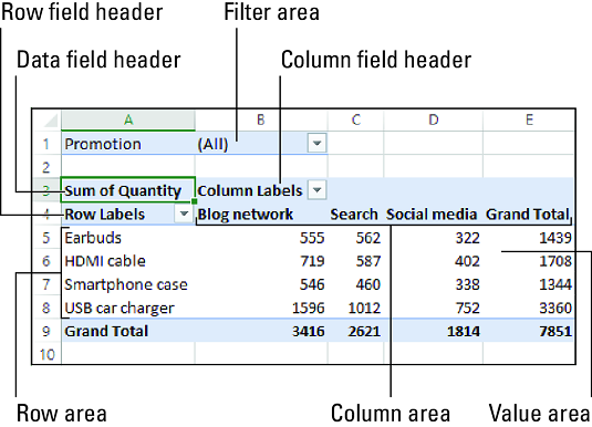 The features of a typical PivotTable.
Find out how to create a PivotTable in Excel 2019.


