


To create a two-variable data table in Excel 2013, you enter two ranges of possible input values for the same formula in the Data Table dialog box: a range of values for the Row Input Cell across the first row of the table and a range of values for the Column Input Cell down the first column of the table.
You then enter the formula (or a copy of it) in the cell located at the intersection of this row and column of input values.
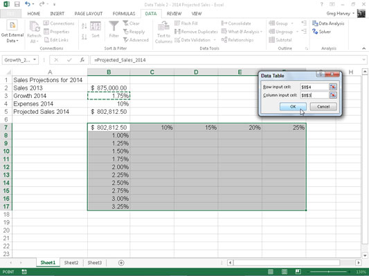
This version of the projected sales spreadsheet uses two variables to calculate the projected sales for year 2014: a growth rate as a percentage of increase over last year’s sales (in cell B3 named Growth_2014) and expenses calculated as a percentage of last year’s sales (in cell B4 named Expenses_2014). In this example, the original formula created in cell B5 is a bit more complex:
=Sales_2013+(Sales_2013*Growth_2014) - (Sales_2013*Expenses_2014)
To set up the two-variable data table, add a row of possible Expenses_2014 percentages in the range C7:F7 to a column of possible Growth_2014 percentages in the range B8:B17.Then, copy the original formula named Projected_Sales_2014 from cell B5 to cell B7, the cell at the intersection of this row of Expenses_2014 percentages and column of Growth_2014 percentages with the formula:
=Projected_Sales_2014
With these few steps, you can create a two-variable data table :
Select the cell range B7:F17.
This cell range incorporates the copy of the original formula along with the row of possible expenses and growth-rate percentages.

Click Data→What-If Analysis→Data Table on the Ribbon.
Excel opens the Data Table dialog box with the insertion point in the Row Input Cell text box.
Click cell B4 to enter the absolute cell address, $B$4, in the Row Input Cell text box.
Click the Column Input Cell text box and then click cell B3 to enter the absolute cell address, $B$3, in this text box.
Click OK to close the Data Table dialog box.
Excel fills the blank cells of the data table with a TABLE formula using B4 as the Row Input Cell and B3 as the Column Input Cell.
Click cell B7, then click the Format Painter command button in the Clipboard group on the Home tab and drag through the cell range C8:F17 to copy the Accounting number format with no decimal places to this range.
This Accounting number format is too long to display given the current width of columns C through F — indicated by the ###### symbols. With the range C8:F17 still selected from using the Format Painter, Step 7 fixes this problem.
Click the Format command button in the Cells group of the Home tab and then click AutoFit Column Width on its drop-down menu.
The array formula {=TABLE(B4,B3)} that Excel creates for the two-variable data table in this example specifies both a Row Input Cell argument (B4) and a Column Input Cell argument (B3). (See the nearby “Array formulas and the TABLE function in data tables” sidebar.) Because this single array formula is entered into the entire data table range of C8:F17, any editing is restricted to this range.


