

| X1 | X2 | X3 | Y1 |
| 0 | 0 | 0 | 1 |
| 0 | 0 | 1 | 0 |
| 0 | 1 | 0 | 0 |
| 0 | 1 | 1 | 0 |
| 1 | 0 | 0 | 0 |
| 1 | 0 | 1 | 0 |
| 1 | 1 | 0 | 0 |
| 1 | 1 | 1 | 1 |
The neural-net Python code
Here, you will be using the Python library called NumPy, which provides a great set of functions to help organize a neural network and also simplifies the calculations.Our Python code using NumPy for the two-layer neural network follows. Using nano (or your favorite text editor), open up a file called “2LayerNeuralNetwork.py” and enter the following code:
# 2 Layer Neural Network in NumPy
import numpy as np
# X = input of our 3 input XOR gate
# set up the inputs of the neural network (right from the table)
X = np.array(([0,0,0>,[0,0,1>,[0,1,0>, \
[0,1,1>,[1,0,0>,[1,0,1>,[1,1,0>,[1,1,1>), dtype=float)
# y = our output of our neural network
y = np.array(([1>, [0>, [0>, [0>, [0>, \
[0>, [0>, [1>), dtype=float)
# what value we want to predict
xPredicted = np.array(([0,0,1>), dtype=float)
X = X/np.amax(X, axis=0) # maximum of X input array
# maximum of xPredicted (our input data for the prediction)
xPredicted = xPredicted/np.amax(xPredicted, axis=0)
# set up our Loss file for graphing
lossFile = open("SumSquaredLossList.csv", "w")
class Neural_Network (object):
def __init__(self):
#parameters
self.inputLayerSize = 3 # X1,X2,X3
self.outputLayerSize = 1 # Y1
self.hiddenLayerSize = 4 # Size of the hidden layer
# build weights of each layer
# set to random values
# look at the interconnection diagram to make sense of this
# 3x4 matrix for input to hidden
self.W1 = \
np.random.randn(self.inputLayerSize, self.hiddenLayerSize)
# 4x1 matrix for hidden layer to output
self.W2 = \
np.random.randn(self.hiddenLayerSize, self.outputLayerSize)
def feedForward(self, X):
# feedForward propagation through our network
# dot product of X (input) and first set of 3x4 weights
self.z = np.dot(X, self.W1)
# the activationSigmoid activation function - neural magic
self.z2 = self.activationSigmoid(self.z)
# dot product of hidden layer (z2) and second set of 4x1 weights
self.z3 = np.dot(self.z2, self.W2)
# final activation function - more neural magic
o = self.activationSigmoid(self.z3)
return o
def backwardPropagate(self, X, y, o):
# backward propagate through the network
# calculate the error in output
self.o_error = y - o
# apply derivative of activationSigmoid to error
self.o_delta = self.o_error*self.activationSigmoidPrime(o)
# z2 error: how much our hidden layer weights contributed to output
# error
self.z2_error = self.o_delta.dot(self.W2.T)
# applying derivative of activationSigmoid to z2 error
self.z2_delta = self.z2_error*self.activationSigmoidPrime(self.z2)
# adjusting first set (inputLayer --> hiddenLayer) weights
self.W1 += X.T.dot(self.z2_delta)
# adjusting second set (hiddenLayer --> outputLayer) weights
self.W2 += self.z2.T.dot(self.o_delta)
def trainNetwork(self, X, y):
# feed forward the loop
o = self.feedForward(X)
# and then back propagate the values (feedback)
self.backwardPropagate(X, y, o)
def activationSigmoid(self, s):
# activation function
# simple activationSigmoid curve as in the book
return 1/(1+np.exp(-s))
def activationSigmoidPrime(self, s):
# First derivative of activationSigmoid
# calculus time!
return s * (1 - s)
def saveSumSquaredLossList(self,i,error):
lossFile.write(str(i)+","+str(error.tolist())+'\n')
def saveWeights(self):
# save this in order to reproduce our cool network
np.savetxt("weightsLayer1.txt", self.W1, fmt="%s")
np.savetxt("weightsLayer2.txt", self.W2, fmt="%s")
def predictOutput(self):
print ("Predicted XOR output data based on trained weights: ")
print ("Expected (X1-X3): \n" + str(xPredicted))
print ("Output (Y1): \n" + str(self.feedForward(xPredicted)))
myNeuralNetwork = Neural_Network()
trainingEpochs = 1000
#trainingEpochs = 100000
for i in range(trainingEpochs): # train myNeuralNetwork 1,000 times
print ("Epoch # " + str(i) + "\n")
print ("Network Input : \n" + str(X))
print ("Expected Output of XOR Gate Neural Network: \n" + str(y))
print ("Actual Output from XOR Gate Neural Network: \n" + \
str(myNeuralNetwork.feedForward(X)))
# mean sum squared loss
Loss = np.mean(np.square(y - myNeuralNetwork.feedForward(X)))
myNeuralNetwork.saveSumSquaredLossList(i,Loss)
print ("Sum Squared Loss: \n" + str(Loss))
print ("\n")
myNeuralNetwork.trainNetwork(X, y)
myNeuralNetwork.saveWeights()
myNeuralNetwork.predictOutput()
Breaking down the Python code for a neural network
Some of the following Python code is a little obtuse the first time through, so here are some explanations.# 2 Layer Neural Network in NumPy import numpy as npIf you get an import error when running the preceding code, install the NumPy Python library. To do so on a Raspberry Pi (or an Ubuntu system), type the following in a terminal window:
sudo apt-get install python3-numpyNext, all eight possibilities of the X1–X3 inputs and the Y1 output are defined.
# X = input of our 3 input XOR gate
# set up the inputs of the neural network (right from the table)
X = np.array(([0,0,0>,[0,0,1>,[0,1,0>, \
[0,1,1>,[1,0,0>,[1,0,1>,[1,1,0>,[1,1,1>), dtype=float)
# y = our output of our neural network
y = np.array(([1>, [0>, [0>, [0>, [0>, \
[0>, [0>, [1>), dtype=float)
In this part of your Python code, you pick a value to predict (this is the particular answer you want at the end).
# what value we want to predict
xPredicted = np.array(([0,0,1>), dtype=float)
X = X/np.amax(X, axis=0) # maximum of X input array
# maximum of xPredicted (our input data for the prediction)
xPredicted = xPredicted/np.amax(xPredicted, axis=0)
Save out our Sum Squared Loss results to a file for use by Excel per epoch.
# set up our Loss file for graphing
lossFile = open("SumSquaredLossList.csv", "w")
FBuild the Neural_Network class for this problem. This image shows the network that is being built.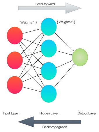 Building a neural network
You can see that each of the layers are represented by a line of Python code in the network.
class Neural_Network (object):
def __init__(self):
#parameters
self.inputLayerSize = 3 # X1,X2,X3
self.outputLayerSize = 1 # Y1
self.hiddenLayerSize = 4 # Size of the hidden layer
Set all the network weights to random values to start.
# build weights of each layer
# set to random values
# look at the interconnection diagram to make sense of this
# 3x4 matrix for input to hidden
self.W1 = \
np.random.randn(self.inputLayerSize, self.hiddenLayerSize)
# 4x1 matrix for hidden layer to output
self.W2 = \
np.random.randn(self.hiddenLayerSize, self.outputLayerSize)
The
feedForward function implements the feed-forward path through the neural network. This basically multiplies the matrices containing the weights from each layer to each layer and then applies the sigmoid activation function.
def feedForward(self, X):
# feedForward propagation through our network
# dot product of X (input) and first set of 3x4 weights
self.z = np.dot(X, self.W1)
# the activationSigmoid activation function - neural magic
self.z2 = self.activationSigmoid(self.z)
# dot product of hidden layer (z2) and second set of 4x1 weights
self.z3 = np.dot(self.z2, self.W2)
# final activation function - more neural magic
o = self.activationSigmoid(self.z3)
return o
And now add the
backwardPropagate function that implements the real trial-and-error learning that our neural network uses.
def backwardPropagate(self, X, y, o):
# backward propagate through the network
# calculate the error in output
self.o_error = y - o
# apply derivative of activationSigmoid to error
self.o_delta = self.o_error*self.activationSigmoidPrime(o)
# z2 error: how much our hidden layer weights contributed to output
# error
self.z2_error = self.o_delta.dot(self.W2.T)
# applying derivative of activationSigmoid to z2 error
self.z2_delta = self.z2_error*self.activationSigmoidPrime(self.z2)
# adjusting first set (inputLayer --> hiddenLayer) weights
self.W1 += X.T.dot(self.z2_delta)
# adjusting second set (hiddenLayer --> outputLayer) weights
self.W2 += self.z2.T.dot(self.o_delta)
To train the network for a particular epoch, you need to call both the
backwardPropagate and the feedForward functions each time you train the network.
def trainNetwork(self, X, y):
# feed forward the loop
o = self.feedForward(X)
# and then back propagate the values (feedback)
self.backwardPropagate(X, y, o)
The
sigmoid activation function and the first derivative of the sigmoid activation function follows.
def activationSigmoid(self, s):
# activation function
# simple activationSigmoid curve as in the book
return 1/(1+np.exp(-s))
def activationSigmoidPrime(self, s):
# First derivative of activationSigmoid
# calculus time!
return s * (1 - s)
Next, save the epoch values of the
loss function to a file for Excel and the neural weights.
def saveSumSquaredLossList(self,i,error):
lossFile.write(str(i)+","+str(error.tolist())+'\n')
def saveWeights(self):
# save this in order to reproduce our cool network
np.savetxt("weightsLayer1.txt", self.W1, fmt="%s")
np.savetxt("weightsLayer2.txt", self.W2, fmt="%s")
Next, run the neural network to predict the outputs based on the current trained weights.
def predictOutput(self):
print ("Predicted XOR output data based on trained weights: ")
print ("Expected (X1-X3): \n" + str(xPredicted))
print ("Output (Y1): \n" + str(self.feedForward(xPredicted)))
myNeuralNetwork = Neural_Network()
trainingEpochs = 1000
#trainingEpochs = 100000
The following is the main training loop that goes through all the requested epochs. Change the variable trainingEpochs above to vary the number of epochs you would like to train your network.
for i in range(trainingEpochs): # train myNeuralNetwork 1,000 times
print ("Epoch # " + str(i) + "\n")
print ("Network Input : \n" + str(X))
print ("Expected Output of XOR Gate Neural Network: \n" + str(y))
print ("Actual Output from XOR Gate Neural Network: \n" + \
str(myNeuralNetwork.feedForward(X)))
# mean sum squared loss
Loss = np.mean(np.square(y - myNeuralNetwork.feedForward(X)))
myNeuralNetwork.saveSumSquaredLossList(i,Loss)
print ("Sum Squared Loss: \n" + str(Loss))
print ("\n")
myNeuralNetwork.trainNetwork(X, y)
Save the results of your training for reuse and predict the output of our requested value.
myNeuralNetwork.saveWeights()
myNeuralNetwork.predictOutput()
Running the neural-network Python code
At a command prompt, enter the following command:python3 2LayerNeuralNetworkCode.pyYou will see the program start stepping through 1,000 epochs of training, printing the results of each epoch, and then finally showing the final input and output. It also creates the following files of interest:
- txt: This file contains the final trained weights for input-layer-to-hidden-layer connections (a 4x3 matrix).
- txt: This file contains the final trained weights for hidden-layer-to-output-layer connections (a 1x4 matrix).
- csv: This is a comma-delimited file containing the epoch number and each loss factor at the end of each epoch. You can use this to graph the results across all epochs.
Epoch # 999
Network Input :
[[0. 0. 0.>
[0. 0. 1.>
[0. 1. 0.>
[0. 1. 1.>
[1. 0. 0.>
[1. 0. 1.>
[1. 1. 0.>
[1. 1. 1.>>
Expected Output of XOR Gate Neural Network:
[[1.>
[0.>
[0.>
[0.>
[0.>
[0.>
[0.>
[1.>>
Actual Output from XOR Gate Neural Network:
[[0.93419893>
[0.04425737>
[0.01636304>
[0.03906686>
[0.04377351>
[0.01744497>
[0.0391143 >
[0.93197489>>
Sum Squared Loss:
0.0020575319565093496
Predicted XOR output data based on trained weights:
Expected (X1-X3):
[0. 0. 1.>
Output (Y1):
[0.04422615><
At the bottom, you see our expected output is 0. 04422615, which is quite close, but not quite, the expected value of 0. If you compare each of the expected outputs to the actual output from the network, you see they all match pretty closely. And every time you run it the results will be slightly different because you initialize the weights with random numbers at the start of the run.
The goal of a neural-network training is not to get it exactly right — only right within a stated tolerance of the correct result. For example, if you said that any output above 0.9 is a 1 and any output below 0.1 is a 0, then our network would have given perfect results.
The Sum Squared Loss is a measure of all the errors of all the possible inputs.
If you graph the Sum Squared Loss versus the epoch number, you get the graph shown in Figure 2-4. You can see that it gets better quite quickly and then it tails off. 1,000 epochs are fine for our stated problem.
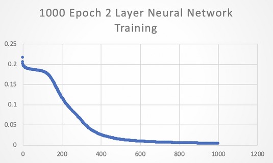 The Loss function during training.
One more experiment. If you increase the number of epochs to 100,000, then the numbers are better still, but our results, according to our accuracy criteria (> 0.9 = 1 and < 0.1 = 0) were good enough in the 1,000 epoch run.
Epoch # 99999
Network Input :
[[0. 0. 0.>
[0. 0. 1.>
[0. 1. 0.>
[0. 1. 1.>
[1. 0. 0.>
[1. 0. 1.>
[1. 1. 0.>
[1. 1. 1.>>
Expected Output of XOR Gate Neural Network:
[[1.>
[0.>
[0.>
[0.>
[0.>
[0.>
[0.>
[1.>>
Actual Output from XOR Gate Neural Network:
[[9.85225608e-01>
[1.41750544e-04>
[1.51985054e-04>
[1.14829204e-02>
[1.17578404e-04>
[1.14814754e-02>
[1.14821256e-02>
[9.78014943e-01>>
Sum Squared Loss:
0.00013715041859631841
Predicted XOR output data based on trained weights:
Expected (X1-X3):
[0. 0. 1.>
Output (Y1):
[0.00014175>
Using TensorFlow for the same neural network
TensorFlow is a Python package that is also designed to support neural networks based on matrices and flow graphs similar to NumPy. It differs from NumPy in one major respect: TensorFlow is designed for use in machine learning and AI applications and so has libraries and functions designed for those applications.TensorFlow gets its name from the way it processes data. A tensor is a multidimensional matrix of data, and this is transformed by each TensorFlow layer it moves through. TensorFlow is extremely Python-friendly and can be used on many different machines and also in the cloud.
Remember, neural networks are data-flow graphs and are implemented in terms of performing operations matrix of data and then moving the resulting data to another matrix. Because matrices are tensors and the data flows from one to another, you can see where the TensorFlow name comes from.
TensorFlow is one of the best-supported application frameworks with APIs (application programming interfaces) gpt Python, C++, Haskell, Java, Go, Rust, and there's also a third-party package for R called tensorflow.
Installing the TensorFlow Python library
For Windows, Linux, and Raspberry Pi, check out the official TensorFlow link.TensorFlow is a typical Python3 library and API (applications programming interface). TensorFlow has a lot of dependencies that will be also installed by following the tutorial referenced above.


