Find the Zero-Input and Zero-State Responses of a Series RC Circuit

To find the total response of an RC series circuit, you need to find the zero-input response and the zero-state response and then add them together. A first-order RC series circuit has one resistor (or network of resistors) and one capacitor connected in series.

Here is an RC series circuit broken up into two circuits. The top-right diagram shows the zero-input response, which you get by setting the input to 0. The bottom-right diagram shows the zero-state response, which you get by setting the initial conditions to 0.

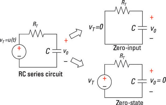
You first want to find the zero-input response for the RC series circuit. The top-right diagram here shows the input signal v_T(t) equal to 0. Zero-input voltage means you have zero . . . nada . . . zip . . . input for all time. The output response is due to the initial condition V₀ (initial capacitor voltage) at time t = 0. The first-order differential equation reduces to

Here, v_ZI(t) is the capacitor voltage. For an input source set to 0 volts as shown here, the capacitor voltage is called a zero-input response or free response. No external forces (such as a battery) are acting on the circuit, except for the initial state of the capacitor voltage.

You can reasonably guess that the solution is the exponential function (you can check and verify the solution afterward). You try an exponential because the time derivative of an exponential is also an exponential. Substitute that guess into the RC first-order circuit equation:

v_ZI(t) =Ae^kt

The A and k are arbitrary constants of the zero-input response. Now substitute the solution v_ZI(t) = Ae^kt into the differential equation:

You get an algebraic characteristic equation after setting the equation equal to 0 and factoring out Ae^kt:

Ae^kt(1 + RCk) = 0

The characteristic equation gives you a much simpler problem. The coefficient of e^kt has to be 0, so you just solve for the constant k:

When you have k, you have the zero-input response v_ZI(t). Using k = –1/RC, you can find the solution to the differential equation for the zero input:

Now you can find the constant A by applying the initial condition. At time t = 0, the initial voltage is V₀, which gives you

The constant A is simply the initial voltage V₀ across the capacitor.

Finally, you have the solution to the capacitor voltage, which is the zero-input response v_ZI(t):

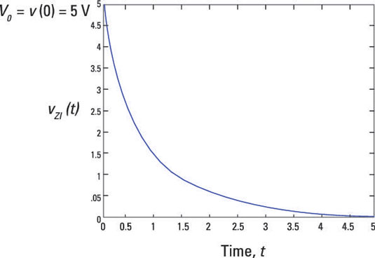
The constant term RC in this equation is called the time constant. The time constant provides a measure of how long a capacitor has discharged or charged. In this example, the capacitor starts at some initial state of voltage V₀ and dissipates quietly into oblivion to another state of 0 volts.

Suppose RC = 1 second and initial voltage V₀ = 5 volts. This sample circuit plots the decaying exponential, showing that it takes about 5 time constants, or 5 seconds, for the capacitor voltage to decay to 0.

Finding the zero-state response by focusing on the input source

Zero-state response means zero initial conditions, and it requires finding the capacitor voltage when there’s an input source, v_T(t). You need to find the homogeneous and particular solutions to get the zero-state response. To find zero initial conditions, you look at the circuit when there’s no voltage across the capacitor at time t = 0.

The circuit at the bottom right of this sample circuit has zero initial conditions and an input voltage of V_T(t) = u(t), where u(t) is a unit step input.

Mathematically, you can describe step function u(t) as

The input signal is divided into two time intervals. When t < 0, u(t) = 0. The first-order differential equation becomes

You’ve already found the solution before time t = 0, because v_h(t) is the solution to the homogeneous equation:

You determine the arbitrary constant c₁ after finding the particular solution and applying the initial condition V₀ of 0 volts.

Now find the particular solution vp(t) when u(t) = 1 after t = 0.

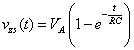
After time t = 0, a unit step input describes the transient voltage behavior across the capacitor. The capacitor voltage reacting to a step input is called the step response.

For a step input v_T(t) = u(t), you have a first-order differential equation:

You already know that the value of the step u(t) is equal to 1 after t = 0. Substitute u(t) = 1 into the preceding equation:

Solve for the capacitor voltage v_p(t), which is the particular solution. The particular solution always depends on the actual input signal.

Because the input is a constant after t = 0, the particular solution v_p(t) is assumed to be a constant V_A as well.

The derivative of a constant is 0, which implies the following:

Now substitute v_p(t) = V_A and its derivative into the first-order differential equation:

After a relatively long period of time, the particular solution follows the unit step input with strength V_A = 1. In general, a step input with strength V_A or V_Au(t) leads to a capacitor voltage of V_A.

After finding the homogeneous and particular solutions, you add up the two solutions to get the zero-state response v_ZS(t). You find c₁ by applying the initial condition that’s equal to 0.

Adding up the homogeneous solution and the particular solution, you have v_ZS(t):

v_ZS(t) = v_h(t) + v_p(t)

Substituting in the homogeneous and particular solutions gives you

At t = 0, the initial condition is v_c(0) = 0 for the zero-state response. You now calculate v_ZS(0) as

Next, solve for c₁:

c₁ = -V_A

Substitute c₁ into the zero-state equation to produce the complete solution of the zero-state response v_ZS(t):