


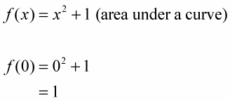
You can approximate the area under a curve by using left sums. For example, say you want the exact area under a curve between two points, 0 and 3. The shaded area on the left graph in the below figure shows the area you want to find.
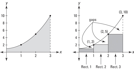
First, you get a rough estimate of the area by drawing three rectangles under the curve, as shown in the right graph in the figure, and then determining the sum of their areas.
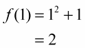
The rectangles in the figure represent a so-called left sum because the upper-left corner of each rectangle touches the curve. Each rectangle has a width of 1 and the height of each is given by the height of the function at the rectangle’s left edge. So, rectangle number 1 has a height of
its area (length x width or height x width) is thus 1 x 1, or 1. Rectangle 2 has a height of
so its area is 2 x 1, or 2. And rectangle 3 has a height of
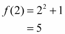
so its area is 5 x 1, or 5. Adding these three areas gives you a total of 1 + 2 + 5, or 8. You can see that this is an underestimate of the total area under the curve because of the three gaps between the rectangles and the curve shown in the above figure.
For a better estimate, double the number of rectangles to six. The following figure shows six “left” rectangles under the curve and also how the six rectangles begin to fill up the three gaps you see in the first figure.
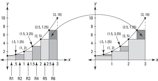
See the three small shaded rectangles in the graph on the right in the second figure? They sit on top of the three rectangles from the first figure, and they represent how much the area estimate has improved by using six rectangles instead of three.
Now total up the areas of the six rectangles. Each has a width of 0.5 and the heights are f(0), f(0.5), f(1), f(1.5), and so on. Here’s the total: 0.5 + 0.625 + 1 + 1.625 + 2.5 + 3.625 = 9.875. This is a better estimate, but it’s still an underestimate because of the six small gaps you can see on the left graph in the above figure.
Here’s the fancy-pants formula for a left rectangle sum. The Left Rectangle Rule: You can approximate the exact area under a curve between a and b,

with the sum of left rectangles given by the following formula. In general, the more rectangles, the better the estimate.
Where n is the number of rectangles,

is the width of each rectangle, and the function values are the heights of the rectangles.
Look back to the six rectangles shown in the second figure. The width of each rectangle equals the length of the total span from 0 to 3 (which of course is 3 – 0, or 3) divided by the number of rectangles, 6. That’s what the
does in the formula.
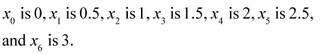
Now, what about those xs with the subscripts? The x-coordinate of the left edge of rectangle 1 in the second figure is called
the right edge of rectangle 1 (which is the same as the left edge of rectangle 2) is at
the right edge of rectangle 2 is at
the right edge of rectangle 3 is at
and so on all the way up to the right edge of rectangle 6, which is at
For the six rectangles in the second figure,
The heights of the six left rectangles in the second figure occur at their left edges, which are at 0, 0.5, 1, 1.5, 2, and 2.5 — that’s
You don’t use the right edge of the last rectangle,
in a left sum. That’s why the list of function values in the formula stops at
Here’s how to use the formula for the six rectangles in the second figure:
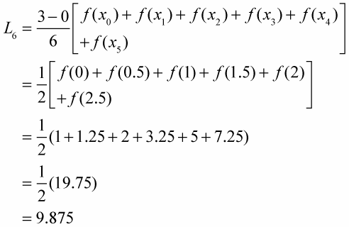
So the area under the curve is 9.875.

