
By the way, if you want to see formulas in cells instead of formula results, go to the Formulas tab and click the Show Formulas button or press Ctrl+’ (apostrophe). Sometimes seeing formulas this way helps to detect formula errors.
Correcting Excel errors one at a time
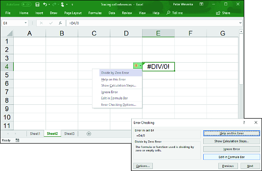
When Excel 2019 detects what it thinks is a formula that has been entered incorrectly, a small green triangle appears in the upper-left corner of the cell where you entered the formula. And if the error is especially egregious, an error message, a cryptic three- or four-letter display preceded by a pound sign (#), appears in the cell.| Message | What Went Wrong |
#DIV/0! |
You tried to divide a number by a zero (0) or an empty cell. |
#NAME |
You used a cell range name in the formula, but the name isn't defined. Sometimes this error occurs because you type the name incorrectly. |
#N/A |
The formula refers to an empty cell, so no data is available for computing the formula. Sometimes people enter N/A in a cell as a placeholder to signal the fact that data isn’t entered yet. Revise the formula or enter a number or formula in the empty cells. |
#NULL |
The formula refers to a cell range that Excel can't understand. Make sure that the range is entered correctly. |
#NUM |
An argument you use in your formula is invalid. |
#REF |
The cell or range of cells that the formula refers to isn't there. |
#VALUE |
The formula includes a function that was used incorrectly, takes an invalid argument, or is misspelled. Make sure that the function uses the right argument and is spelled correctly. |
 Ways to detect and correct errors in Excel.
Running Excel’s error checker
Another way to tackle Excel formula errors is to run the error checker. When the checker encounters what it thinks is an error, the Error Checking dialog box tells you what the error is.To run the error checker, go to the Formulas tab and click the Error Checking button (you may have to click the Formula Auditing button first, depending on the size of your screen).
If you see clearly what the error is, click the Edit in Formula Bar button, repair the error in the Formula bar, and click the Resume button in the dialog box (you find this button at the top of the dialog box). If the error isn't one that really needs correcting, either click the Ignore Error button or click the Next button to send the error checker in search of the next error in your worksheet.
Tracing Excel’s cell references
In a complex worksheet in which Excel formulas are piled on top of one another and the results of some formulas are computed into other formulas, it helps to be able to trace cell references. By tracing cell references, you can see how the data in a cell figures into a formula in another cell; or, if the Excel cell contains a formula, you can see which cells the formula gathers data from to make its computation. You can get a better idea of how your worksheet is constructed, and in so doing, find structural errors more easily.The image below shows how cell tracers describe the relationships between cells. A cell tracer is a blue arrow that shows the relationships between cells used in formulas. You can trace two types of relationships:
- Tracing precedents: Select a cell with a formula in it and trace the formula’s precedents to find out which cells are computed to produce the results of the formula. Trace precedents when you want to find out where a formula gets its computation data. Cell tracer arrows point from the referenced cells to the cell with the formula results in it.
To trace precedents, go to the Formulas tab and click the Trace Precedents button. (You may have to click the Formula Auditing button first, depending on the size of your screen.)
- Tracing dependents: Select a cell and trace its dependents to find out which cells contain formulas that use data from the cell you selected. Cell tracer arrows point from the cell you selected to cells with formula results in them. Trace dependents when you want to find out how the data in a cell contributes to formulas elsewhere in the worksheet. The cell you select can contain a constant value or a formula in its own right (and contribute its results to another formula).
To trace dependents, go to the Formulas tab and click the Trace Dependents button (you may have to click the Formula Auditing button first, depending on the size of your screen).
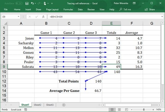 Tracing the relationships between Excel cells.
To remove the cell tracer arrows from a worksheet, go to the Formulas tab and click the Remove Arrows button. You can open the drop-down list on this button and choose Remove Precedent Arrows or Remove Dependent Arrows to remove only cell-precedent or cell-dependent tracer arrows.