


The Iris dataset is not easy to graph for predictive analytics in its original form because you cannot plot all four coordinates (from the features) of the dataset onto a two-dimensional screen. Therefore you have to reduce the dimensions by applying a dimensionality reduction algorithm to the features.
In this case, the algorithm you’ll be using to do the data transformation (reducing the dimensions of the features) is called Principal Component Analysis (PCA).
| Sepal Length | Sepal Width | Petal Length | Petal Width | Target Class/Label |
|---|---|---|---|---|
| 5.1 | 3.5 | 1.4 | 0.2 | Setosa (0) |
| 7.0 | 3.2 | 4.7 | 1.4 | Versicolor (1) |
| 6.3 | 3.3 | 6.0 | 2.5 | Virginica (2) |
The PCA algorithm takes all four features (numbers), does some math on them, and outputs two new numbers that you can use to do the plot. Think of PCA as following two general steps:
It takes as input a dataset with many features.
It reduces that input to a smaller set of features (user-defined or algorithm-determined) by transforming the components of the feature set into what it considers as the main (principal) components.
This transformation of the feature set is also called feature extraction. The following code does the dimension reduction:
>>> from sklearn.decomposition import PCA
>>> pca = PCA(n_components=2).fit(X_train)
>>> pca_2d = pca.transform(X_train)
If you’ve already imported any libraries or datasets, it’s not necessary to re-import or load them in your current Python session. If you do so, however, it should not affect your program.
After you run the code, you can type the pca_2d variable in the interpreter and see that it outputs arrays with two items instead of four. These two new numbers are mathematical representations of the four old numbers. When the reduced feature set, you can plot the results by using the following code:
>>> import pylab as pl
>>> for i in range(0, pca_2d.shape[0]):
>>> if y_train[i] == 0:
>>>  c1 = pl.scatter(pca_2d[i,0],pca_2d[i,1],c='r',    marker='+')
>>> elif y_train[i] == 1:
>>>  c2 = pl.scatter(pca_2d[i,0],pca_2d[i,1],c='g',    marker='o')
>>> elif y_train[i] == 2:
>>>  c3 = pl.scatter(pca_2d[i,0],pca_2d[i,1],c='b',    marker='*')
>>> pl.legend([c1, c2, c3], ['Setosa', 'Versicolor',    'Virginica'])
>>> pl.title('Iris training dataset with 3 classes and    known outcomes')
>>> pl.show()
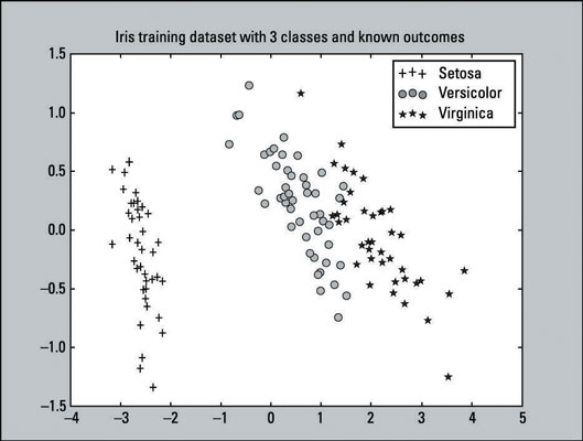
This is a scatter plot — a visualization of plotted points representing observations on a graph. This particular scatter plot represents the known outcomes of the Iris training dataset. There are 135 plotted points (observations) from our training dataset. The training dataset consists of
45 pluses that represent the Setosa class.
48 circles that represent the Versicolor class.
42 stars that represent the Virginica class.
You can confirm the stated number of classes by entering following code:
>>> sum(y_train==0)45
>>> sum(y_train==1)48
>>> sum(y_train==2)42
From this plot you can clearly tell that the Setosa class is linearly separable from the other two classes. While the Versicolor and Virginica classes are not completely separable by a straight line, they’re not overlapping by very much. From a simple visual perspective, the classifiers should do pretty well.
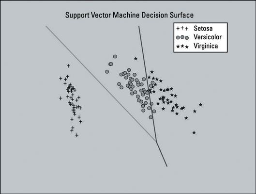
The image below shows a plot of the Support Vector Machine (SVM) model trained with a dataset that has been dimensionally reduced to two features. Four features is a small feature set; in this case, you want to keep all four so that the data can retain most of its useful information. The plot is shown here as a visual aid.
This plot includes the decision surface for the classifier — the area in the graph that represents the decision function that SVM uses to determine the outcome of new data input. The lines separate the areas where the model will predict the particular class that a data point belongs to.
The left section of the plot will predict the Setosa class, the middle section will predict the Versicolor class, and the right section will predict the Virginica class.
The SVM model that you created did not use the dimensionally reduced feature set. This model only uses dimensionality reduction here to generate a plot of the decision surface of the SVM model — as a visual aid.
The full listing of the code that creates the plot is provided as reference. It should not be run in sequence with our current example if you’re following along. It may overwrite some of the variables that you may already have in the session.
The code to produce this plot is based on the sample code provided on the scikit-learn website. You can learn more about creating plots like these at the scikit-learn website.
Here is the full listing of the code that creates the plot:
>>> from sklearn.decomposition import PCA
>>> from sklearn.datasets import load_iris
>>> from sklearn import svm
>>> from sklearn import cross_validation
>>> import pylab as pl
>>> import numpy as np
>>> iris = load_iris()
>>> X_train, X_test, y_train, y_test =   cross_validation.train_test_split(iris.data,   iris.target, test_size=0.10, random_state=111)
>>> pca = PCA(n_components=2).fit(X_train)
>>> pca_2d = pca.transform(X_train)
>>> svmClassifier_2d =   svm.LinearSVC(random_state=111).fit(   pca_2d, y_train)
>>> for i in range(0, pca_2d.shape[0]):
>>> if y_train[i] == 0:
>>>  c1 = pl.scatter(pca_2d[i,0],pca_2d[i,1],c='r',    s=50,marker='+')
>>> elif y_train[i] == 1:
>>>  c2 = pl.scatter(pca_2d[i,0],pca_2d[i,1],c='g',    s=50,marker='o')
>>> elif y_train[i] == 2:
>>>  c3 = pl.scatter(pca_2d[i,0],pca_2d[i,1],c='b',    s=50,marker='*')
>>> pl.legend([c1, c2, c3], ['Setosa', 'Versicolor',   'Virginica'])
>>> x_min, x_max = pca_2d[:, 0].min() - 1,   pca_2d[:,0].max() + 1
>>> y_min, y_max = pca_2d[:, 1].min() - 1,   pca_2d[:, 1].max() + 1
>>> xx, yy = np.meshgrid(np.arange(x_min, x_max, .01),   np.arange(y_min, y_max, .01))
>>> Z = svmClassifier_2d.predict(np.c_[xx.ravel(),  yy.ravel()])
>>> Z = Z.reshape(xx.shape)
>>> pl.contour(xx, yy, Z)
>>> pl.title('Support Vector Machine Decision Surface')
>>> pl.axis('off')
>>> pl.show()