


By performing what-if analyses with Excel 2016 data tables, you change the data in input cells and observe what effect changing the data has on the results of a formula. With a data table, you can experiment simultaneously with many different input cells and in so doing experiment with many different scenarios.
Using a one-input table for analysis
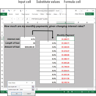
In a one-input table, you find out what the different results of a formula would be if you changed one input cell in the formula. Here, that input cell is the interest rate on a loan. The purpose of this data table is to find out how monthly payments on a $250,000, 30-year mortgage are different, given different interest rates. The interest rate in cell B4 is the input cell.
Follow these steps to create a one-input table:
On your worksheet, enter values that you want to substitute for the value in the input cell.
To make the input table work, you have to enter the substitute values in the right location:
In a column: Enter the values in the column starting one cell below and one cell to the left of the cell where the formula is located. In the example shown, the formula is in cell E4 and the values are in the cell range D5:D15.
In a row: Enter the values in the row starting one cell above and one cell to the right of the cell where the formula is.
Select the block of cells with the formula and substitute values.
Select a rectangle of cells that encompasses the formula cell, the cell beside it, all the substitute values, and the empty cells where the new calculations will soon appear.
In a column: Select the formula cell, the cell to its left, all the substitute-value cells, and the cells below the formula cell.
In a row: Select the formula cell, the cell above it, the substitute values in the cells directly to the right, and the now-empty cells where the new calculations will appear.
On the Data tab, click the What-If Analysis button and choose Data Table on the drop-down list.
You see the Data Table dialog box.
In the Row Input Cell or Column Input Cell text box, enter the address of the cell where the input value is located.
To enter this cell address, go outside the Data Table dialog box and click the cell. The input value is the value you're experimenting with in your analysis. In the case of the worksheet shown, the input value is located in cell B4, the cell that holds the interest rate.
If the new calculations appear in rows, enter the address of the input cell in the Row Input Cell text box; if the calculations appear in columns, enter the input cell address in the Column Input Cell text box.
Click OK.
Excel performs the calculations and fills in the table.
To generate the one-input table, Excel constructs an array formula with the TABLE function. If you change the cell references in the first row or plug in different values in the first column, Excel updates the one-input table automatically.
Using a two-input table for analysis
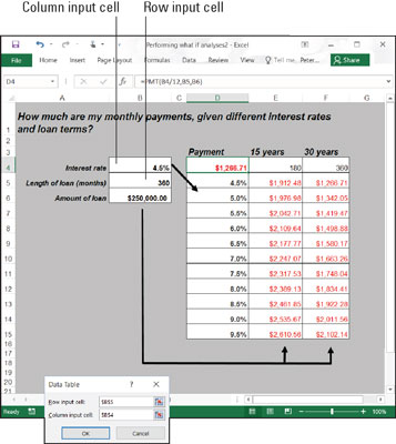
In a two-input table, you can experiment with two input cells rather than one. Getting back to the example of the loan payment, you can calculate not only how loan payments change as interest rates change but also how payments change if the life of the loan changes. This figure shows a two-input table for examining monthly loan payments given different interest rates and two different terms for the loan, 15 years (180 months) and 30 years (360 months).
Follow these steps to create a two-input data table:
Enter one set of substitute values below the formula in the same column as the formula.
Here, different interest rates are entered in the cell range D5:D15.
Enter the second set of substitute values in the row to the right of the formula.
Here, 180 and 360 are entered. These numbers represent the number of months of the life of the loan.
Select the formula and all substitute values.
Do this correctly and you select three columns, including the formula, the substitute values below it, and the two columns to the right of the formula. You select a big block of cells (the range D4:F15, in this example).
On the Data tab, click the What-If Analysis button and choose Data Table on the drop-down list.
The Data Table dialog box appears.
In the Row Input Cell text box, enter the address of the cell referred to in the original formula where substitute values to the right of the formula can be plugged in.
Enter the cell address by going outside the dialog box and selecting a cell. Here, for example, the rows to the right of the formula are for length of loan substitute values. Therefore, select cell B5, the cell referred to in the original formula where the length of the loan is listed.
In the Column Input Cell text box, enter the address of the cell referred to in the original formula where substitute values below the formula are.
The substitute values below the formula cell are interest rates. Therefore, select cell B4, the cell referred to in the original formula where the interest rate is entered.
Click OK.
Excel performs the calculations and fills in the table.


