


Sometimes, none of the pivot tables that Excel 2016 suggests when creating a new table with the Quick Analysis tool or the Recommended PivotTables command button fit the type of data summary you have in mind.
In such cases, you can either select the suggested pivot table whose layout is closest to what you have in mind, or you can choose to create the pivot table from scratch (a process that isn't all that difficult or time consuming).
To manually create a new pivot table from the worksheet with the data to be analyzed, position the cell pointer somewhere in the cells of this list, and then click the PivotTable command button on the Ribbon's Insert tab or press Alt+NV.
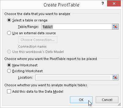
Excel then opens the Create PivotTable dialog box and selects all the data in the list containing the cell cursor (indicated by a marquee around the cell range). You can then adjust the cell range in the Table/Range text box under the Select a Table or Range button if the marquee does not include all the data to summarize in the pivot table.
By default, Excel builds the new pivot table on a new worksheet it adds to the workbook. If, however, you want the pivot table to appear on the same worksheet, click the Existing Worksheet button and then indicate the location of the first cell of the new table in the Location text box, as shown here. (Just be sure that this new pivot table isn't going to overlap any existing tables of data.)
If the data source for your pivot table is an external database table created with a separate database management program, such as Access, you need to click the Use an External Data Source button, click the Choose Connection button, and then click the name of the connection in the Existing Connections dialog box.
Also, Excel 2016 supports analyzing data from multiple related tables on a worksheet (referred to as a Data Model). If the data in new pivot table you're creating is to be analyzed along with another existing pivot table, be sure to select the Add This Data to the Data Model check box.
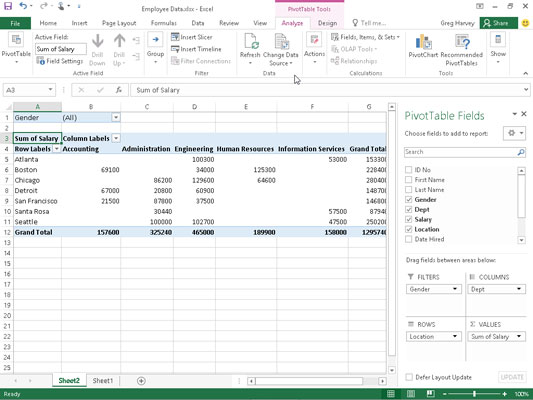
If you indicate a new worksheet as the location for the new pivot table in the Create PivotTable dialog box, when you click OK, the program inserts a new worksheet at the front of the workbook with a blank grid for the new pivot table. It also opens a PivotTable Fields task pane on the right side of the Worksheet area and adds the PivotTable Tools contextual tab to the Ribbon (see the following figure).
The PivotTable Fields task pane is divided into two areas: the Choose Fields to Add to Report list box with the names of all the fields in the data list you can select as the source of the table preceded by empty check boxes, and a Drag Fields between Areas Below section divided into four drop zones (FILTERS, COLUMNS, ROWS, and VALUES).
You can also insert a new worksheet with the blank pivot table grid like the one shown by selecting the Blank PivotTable button in the Recommended PivotTable dialog box or the Quick Analysis tool's options palette (displayed only when Quick Analysis can't suggest pivot tables for your data). Just be aware that when you select the Blank PivotTable button in this dialog box or palette, Excel 2016 does not first open the Create PivotTable dialog box.
If you need to use any of the options offered in this dialog box in creating your new pivot table, you need to create the pivot table with the PivotTable command button rather than the Recommended PivotTables command button on the Insert Tab.
To complete the new pivot table, all you have to do is assign the fields in the PivotTable Fields task pane to the various parts of the table. You do this by dragging a field name from the Choose Fields to Add to Report list box and dropping it in one of the four areas below called drop zones:
FILTERS: This area contains the fields that enable you to page through the data summaries shown in the actual pivot table by filtering out sets of data — they act as the filters for the report. For example, if you designate the Year field from a data list as a report filter, you can display data summaries in the pivot table for individual years or for all years represented in the data list.
COLUMNS: This area contains the fields that determine the arrangement of data shown in the columns of the pivot table.
ROWS: This area contains the fields that determine the arrangement of data shown in the rows of the pivot table.
VALUES: This area contains the fields that determine which data are presented in the cells of the pivot table — they are the values that are summarized in its last column (totaled by default).
To understand how these various zones relate to a pivot table, look at the completed pivot table shown.
For this pivot table, the Gender field from the data list (a field that contains F [for female] or M [for male]) is assigned to indicate the employee's gender in the FILTERS drop zone. The Dept field (that contains the names of the various departments in the company) is assigned to the COLUMNS drop zone, the Location field (that contains the names of the various cities with corporate offices) to the ROWS drop zone, and the Salary field to the VALUES drop zone.
As a result, this pivot table now displays the sum of the salaries for both the male and female employees in each department (across the columns) and then presents these sums by their corporate location (in each row).
As soon as you add fields to a new pivot table (or select the cell of an existing table in a worksheet), Excel selects the Analyze tab of the PivotTable Tools contextual tab that automatically appears in the Ribbon. Among the many groups on this tab, you find the Show group at the end that contains the following useful command buttons:
Field List to hide and redisplay the PivotTable Field List task pane on the right side of the Worksheet area
+/− Buttons to hide and redisplay the expand (+) and collapse (–) buttons in front of particular column fields or row fields that enable you to temporarily remove and then redisplay their particular summarized values in the pivot table
Field Headers to hide and redisplay the fields assigned to the Column Labels and Row Labels in the pivot table


