


Excel 2013 makes it simple to create a new pivot table using a data list selected in your worksheet with its new Quick Analysis tool. To preview various types of pivot tables that Excel can create for you on the spot using the entries in a data list that you have open in an Excel worksheet, simply follow these steps:
Select all the data (including the column headings) in your data list as a cell range in the worksheet.
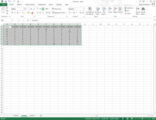
If you’ve assigned a range name to the data list, you can select the column headings and all the data records in one operation simply by choosing the data list’s name from the Name box drop-down menu.
Click the Quick Analysis tool that appears right below the lower-right corner of the current cell selection.
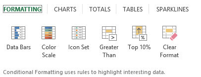
Doing this opens the palette of Quick Analysis options with the initial Formatting tab selected and its various conditional formatting options displayed.
Click the Tables tab at the top of the Quick Analysis options palette.
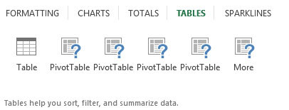
Excel selects the Tables tab and displays its Table and PivotTable option buttons. The Table button previews how the selected data would appear formatted as a table. The other PivotTable buttons preview the various types of pivot tables that can be created from the selected data.
To preview each pivot table that Excel 2013 can create for your data, highlight its PivotTable button in the Quick Analysis palette.
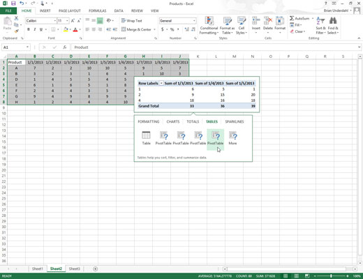
As you highlight each PivotTable button in the options palette, Excel’s Live Preview feature displays a thumbnail of a pivot table that can be created using your table data. This thumbnail appears above the Quick Analysis options palette for as long as the mouse or Touch pointer is over its corresponding button.
When a preview of the pivot table you want to create appears, click its button in the Quick Analysis options palette to create it.

Excel 2013 then creates the previewed pivot table on a new worksheet that is inserted at the beginning of the current workbook. This new worksheet containing the pivot table is active so that you can immediately rename and relocate the sheet as well as edit the new pivot table, if you wish.


