


Excel 2013 supports a wide variety of built-in functions that you can use when building formulas. Of course, the most popular built-in function is by far the SUM function, which is automatically inserted when you click the Sum command button on the Home tab of the Ribbon.
(Keep in mind that you can also use this drop-down button attached to the Sum button to insert the AVERAGE, COUNT, MAX, and MIN functions.) To use other Excel functions, you can use the Insert Function button on the Formula bar (the one with the fx).
When you click the Insert Function button, Excel displays the Insert Function dialog box. You can then use its options to find and select the function that you want to use and to define the argument or arguments that the function requires in order to perform its calculation.

To select the function that you want to use, you can use any of the following methods:
Click the function name if it’s one that you’ve used lately and is therefore already listed in the Select a Function list box.
Select the name of the category of the function that you want to use from the Or Select a Category drop-down list box (Most Recently Used is the default category) and then select the function that you want to use in that category from the Select a Function list box.
Replace the text “Type a brief description of what you want to do and then click Go” in the Search for a Function text box with keywords or a phrase about the type of calculation that you want to do (such as “return on investment”). Click the Go button or press Enter and click the function that you want to use in the Recommended category displayed in the Select a Function list box.
When selecting the function to use in the Select a Function list box, click the function name to have Excel give you a short description of what the function does, displayed underneath the name of the function with its argument(s) shown in parentheses (referred to as the function’s syntax).
To get help on using the function, click the Help on This Function link displayed in the lower-left corner of the Insert Function dialog box to open the Help window in its own pane on the right. When you finish reading and/or printing this help topic, click the Close button to close the Help window and return to the Insert Function dialog box.
You can select the most commonly used types of Excel functions and enter them simply by choosing their names from the drop-down menus attached to their command buttons in the Function Library group of the Formulas tab of the Ribbon. These command buttons include Financial, Logical, Text, Date & Time, Lookup & Reference, and Math & Trig.
In addition, you can select functions in the Statistical, Engineering, Cube, Information, Compatibility, and Web categories from continuation menus that appear when you click the More Functions command button on the Formulas tab.
And if you find you need to insert a function in the worksheet that you recently entered into the worksheet, chances are good that when you click the Recently Used command button, that function will be listed on its drop-down menu for you to select.
When you click OK after selecting the function that you want to use in the current cell, Excel inserts the function name followed by a closed set of parentheses on the Formula bar. At the same time, the program closes the Insert Function dialog box and then opens the Function Arguments dialog box.
You then use the argument text box or boxes displayed in the Function Arguments dialog box to specify what numbers and other information are to be used when the function calculates its result.
All functions — even those that don’t take any arguments, such as the TODAY function — follow the function name by a closed set of parentheses, as in =TODAY(). If the function requires arguments (and almost all require at least one), these arguments must appear within the parentheses following the function name.
When a function requires multiple arguments, such as the DATE function, the various arguments are entered in the required order (as in year, month, day for the DATE function) within the parentheses separated by commas, as in DATE(33,7,23).
When you use the text boxes in the Function Arguments dialog box to input the arguments for a function, you can select the cell or cell range in the worksheet that contains the entries that you want used.
Click the text box for the argument that you want to define and then either start dragging the cell cursor through the cells or, if the Function Arguments dialog box is obscuring the first cell in the range that you want to select, click the Collapse Dialog Box button located to the immediate right of the text box.
Dragging or clicking this button reduces the Function Arguments dialog box to just the currently selected argument text box, thus enabling you to drag through the rest of the cells in the range.
If you started dragging without first clicking the Collapse Dialog Box button, Excel automatically expands the Function Arguments dialog box as soon as you release the mouse button.
If you clicked the Collapse Dialog Box button, you have to click the Expand Dialog Box button (which replaces the Collapse Dialog Box button located to the right of the argument text box) in order to restore the Function Arguments dialog box to its original size.
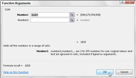
As you define arguments for a function in the Function Arguments dialog box, Excel shows you the calculated result following the heading, “Formula result =” near the bottom of the Function Arguments dialog box.
When you finish entering the required argument(s) for your function (and any optional arguments that may pertain to your particular calculation), click OK to have Excel close the Function Arguments dialog box and replace the formula in the current cell display with the calculated result.
You can also type the name of the function instead of selecting it from the Insert Function dialog box. When you begin typing a function name after typing an equal sign (=), Excel’s AutoComplete feature kicks in by displaying a drop-down menu with the names of all the functions that begin with the character(s) you type.
You can then enter the name of the function you want to use by double-clicking its name on this drop-down menu. Excel then enters the function name along with the open parenthesis as in =DATE( so that you can then begin selecting the cell range(s) for the first argument.


