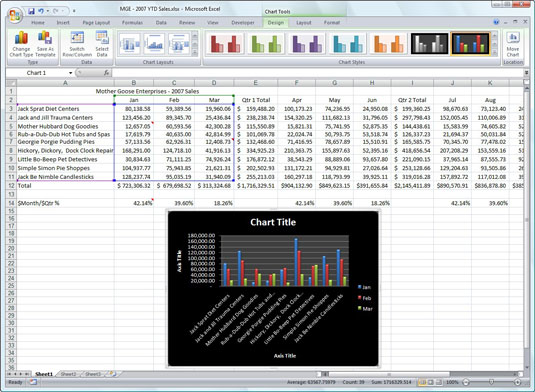
When you add a chart to an Excel 2007 workbook, a new Chart Tools Design tab appears in the Ribbon. You can use the command buttons on the Chart Tools Design tab to customize the chart type and style. The Design tab contains the following groups of buttons:
Type group
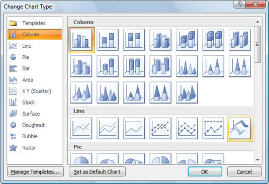
Click the Change Chart Type button to change the type of chart, for example, to change from a bar chart to a line chart or a pie graph. Just click the thumbnail of the new chart type in the Change Chart Type dialog box.
Click the Save As Template button to open the Save Chart Template dialog box, where you save the current chart’s formatting and layout (usually after customizing) as a template to use in creating future charts.
Data group
Click the Switch Row/Column button to immediately transpose the worksheet data used for the Legend Entries (Series) and that used for the Axis Labels (Categories) in the selected chart.
Click the Select Data button to open the Select Data Source dialog box, where you can not only transpose the Legend Entries (Series) and the Axis Labels (Categories) but also edit out or add particular entries to either category.
Chart Layouts group
Click the More button (the last one with the horizontal bar and triangle pointing downward) to display all the thumbnails on the Chart Layouts drop-down gallery. Then click the thumbnail of the new layout style you want applied to the selected chart.
Chart Styles group
Click the More button (the last one with the horizontal bar and triangle pointing downward) to display all the thumbnails on the Chart Styles drop-down gallery. Then click the thumbnail of the new chart style you want applied to the selected chart.
Note that the Chart Layout and the Chart Styles galleries do not use the Live Preview feature. This means that you have to click a thumbnail in the gallery and actually apply it to the selected chart in order to see how it looks.