
Computer tools play a big part in modern signals and systems analysis and design. LCC differential and difference equations are a fundamental part of simple and highly complex systems. Fortunately, current software tools make it possible to work across domains with these LCC equations without too much pain.
LCC differential and difference equations are completely characterized by the {ak} and {bk} coefficient sets. You can use such tools as Pylab with the SciPy signal package to design high performance filters, particularly in the discrete-time domain. The filter design functions of signal give you the {ak} and {bk} coefficients in response to the design requirements you input. You can then use the filter designs in the simulation of larger systems.
Continuous time
Three representations of the LCC differential equation system are the time, frequency, and s-domains, and the same coefficient sets, {bk} and {ak}, exist in all three representations. Here are the corresponding input and output relationships in these domains:
Time domain (from differential equation):
Time domain (from impulse response):
Frequency domain:
s-domain:
In the second line of the differential equation, the impulse response, h(t), along with the convolution integral produce the output, y(t), from the input, x(t). In the third line, the convolution theorem for Fourier transforms produces the output spectrum, Y(f), as the product of the input spectrum, X(f), and the frequency response, H(f) — which is the Fourier transform of the impulse response.
In the fourth line, the convolution theorem for Laplace transforms produces the s-domain output, Y(s), as the product of the input, X(s), and the system function, H(s) — which is the Laplace transform of the impulse response.
The figurehighlights the key functions in PyLab and the ssd.py code module you can use to work across continuous-time domains. Remember, these functions are at the top level. You can integrate many lower-level functions (such as math, array manipulation, and plotting library functions) with these top-level functions to carry out specific analysis tasks.
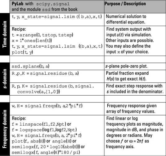
Here’s what you can find:
The time-domain rows show a recipe to solve the differential equation numerically by using signal.lsim((b,a),x,t) for a step function input. The arrays b and a correspond to the coefficient sets {bk} and {ak}. Input signals of your own choosing are possible, too. The time-domain simulation allows you to characterize a system’s behavior at the actual waveform level.
In the s-domain rows, find the pole-zero plot of the system function H(s) by using ssd.splane(b,a). Also find out how to solve the partial fraction expansion (PFE) of H(s) and H(s)/s to get a mathematical representation of the impulse response or the step response.
The frequency-domain section offers a recipe for plotting the frequency response of the system by using signal.freqs(b,a,2*pi*f). Options include a linear or log frequency axis, the frequency response magnitude, and the phase response in degrees.
Discrete time
Just like for differential equation systems described in the previous section, the LCC difference equation system has three representations: time, frequency, and z-domains, and the same coefficient sets, {bk} and {ak}, exist in all three representations. Here are the corresponding input and output relationships in these domains:
Time domain (from difference equation):
Time domain (from impulse response):
Frequency domain:
z-domain:
In the second line of the difference equation, the impulse response, h[n], along with the convolution sum produce the output, y[n], form the input, x[n]. In the third line, the convolution theorem for Fourier transforms produces the output spectrum,
which is the discrete-time Fourier transform of the impulse response.
In the fourth line, the convolution theorem for z-transforms produces the z-domain output, Y(z), as the product of the input, X(z), and the system function, H(z), which is the z-transform of the impulse response.
The figure highlights the key functions in PyLab and the custom ssd.py code module you can use to work across discrete-time domains.
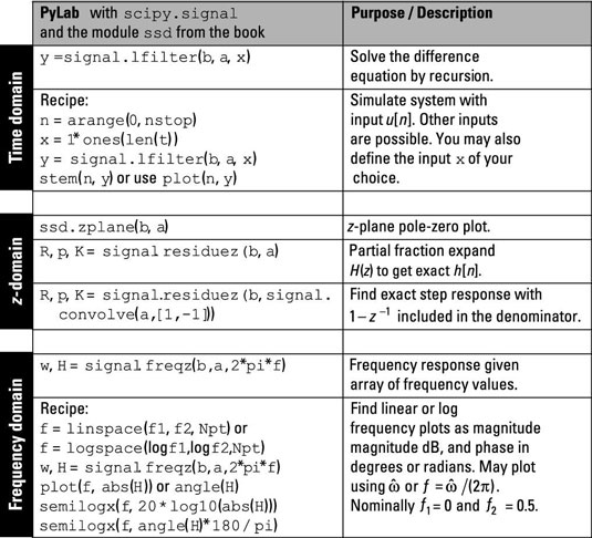
In the time domain rows, you solve the difference equation exactly, using signal.lfilter(b,a,x).
In the z-domain rows, you can find the pole-zero plot of the system function H(z), using ssd.zplane(b,a), and the partial fraction expansion, using signal.residuez instead of signal.residue.
The frequency domain rows show you how to find the frequency response of a discrete-time system with signal.freqz(b,a,2*pi*f), where f is the frequency variable